| Overview | All Modules | Tutorial | User's Guide | Programming Guide |
Module category: IO
ReadPAM reads DSY and THP files. From the DSY file it may read the grid, nodal and cell data. Global data may be read from either the DSY file or the THP. Before you try using this module and the examples below you have to set the PAMHOME environment variable. A line setting this variable may be already present in your .covise file. In this case you may have to correct the value for this variable to the path of the directory for your DSY library installation directory. Your license file, without which this module will not work, is found in the subdirectory licenses under this directory.
The module inspects the input file and produces lists for the available variables that you may select for output. The number of cell or global variables may be sometimes very long. There should be no problem with that in principle, but in extreme cases, some important time delays may appear. Then you may limit the number of the different categories of variables by creating a ReadPAM_Limits section in your covise.config file. In this section you may define the following variables:
We strongly recommend not to use this section in your covise.config unless it is extremely necessary. If you create this section thereby establishing some limits, and create a map with them, in the future you will have to use the same limits in order to run successfully that net file, otherwise ReadPAM will probably crash.
An additional remark about long choice lists is in order. You may have difficulties when trying to access some variable if the choice list is too long for the dimensions of your screen. That is not a real problem, you may also change the appearance of the parameter to a combo box.
ReadPAM is available for COVISE version 5.1 and higher. It has been tested on SGI systems (IRIX 6.5).
SGI only, PAM license required - no LINUX support
| Name | Type | Description |
| DSY_file | File Browser | DSY file (used mainly for visualisation). |
| THP_file | File Browser | THP file (used mainly for global or non-local data). |
| scale | Scalar | You may modify the default valule (1.0) in order to amplify or suppress the deformation of the grid. |
| timeSteps | Vector | When you set a DSY file, the components of this vector are automatically set with some default values: the first component is the initial time step for visualisation, and its default value is 1; the second component is the final time step for visualisation and its default value is the number of time steps that have been stored in the file; with the third component you may jump between time steps, the default value is 1, which means that all time steps between the first and the last one that you wish to visualise are read, a value of 2 means that only every second time step is read, and so forth. The time step indicated by the first component is always read in. |
| Nodal_Var1
Nodal_Var2 | Choice | Selection of nodal magnitude. |
| Cell_Var1
Cell_Var2 | Choice | Selection of element-based magnitude. |
| DSY_or_THP | Boolean | This is only relevant for global variables. When this switch is true, then global variables are read from the DSY file. When it is false, from the THP file. |
| Global_Var1...
Global_Var6 | Choice | Selection of non-local variables. These data are not intended for visualisation with a renderer, but with the Plot module. |
| Port select | switch | You may output tensor objects out of cell-based fields. In order to do that you activate one of the options: Tensor port 1 or Tensor port 2. Then there will appear on the control panel a list of 9 choice parameters for a maximum of 9 components. You may produce tensors of 4 types: symmetric 2D (3 independent components), full 2D (4 independent components), symmetric 3D (6 independent components) and full 3D (9 independnet components). For the 2D cases only the XX, XY, YX, and YY are relevant. If you want to produce a symmetric tensor, it is not necessary to repeat a redundant component. |
| T1_Component_XX...
T1_Component_ZZ | Choice | See parameter Port select. These are the components for the object of the first tensor port. |
| T2_Component_XX...
T2_Component_ZZ | Choice | See parameter Port select. These are the components for the object of the second tensor port. |
|
|
| Name | Type | Description |
| outputmeshOut | UnstructuredGrid |
In general you will get a hierarchy of sets.
On the first level you get a set with time steps. The
elements of this set are in their turn sets of unstructured
grids. All elements in each one of these grids are of a unique
type. So you get separate grids according to the element type
of their elements:
|
| outputnodalData1
nodalData2 | Float Vec3 | Data per node. |
| outputcellData1
cellData2 | Float Vec3 | Data per cell. |
| outputglobalData1
globalData2 | Float Vec3 | Non-local data. This category may include:
|
| outputtensorData1 | Unstructured_T3D_Data | Tensor cell-based data. See parameter Port select for more details. |
|
| ||
| outputMaterials | IntArr | A set of sets with the same structure as the grid, but instead of grids, the final set elements are integer arrays storing the material labels for the grid elements. You may find this object useful to visualise parts of the grid using AssembleUsg . |
| outputElem_Labels | IntArr | A set of sets with the same structure as the grid, but instead of grids, the final set elements are integer arrays storing the element labels for the grid elements. You may find this object useful to visualise parts of the grid using AssembleUsg . |
|
|
Some variables of some one-dimensional elements may be vectors defined in the global coordinate reference system or in a local one. In the first case the label for this variable in the choice lists will be terminated with gVEC; in the latter case, with lVEC.
In order to help you identify which kind of element some particular variable is defined for in the case of some exotic one-dimensional elements, we include in the termination of the variable title between parenthesis the following tags:
We present below two examples.
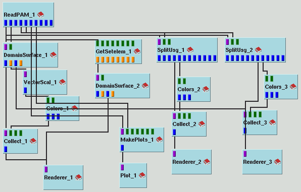
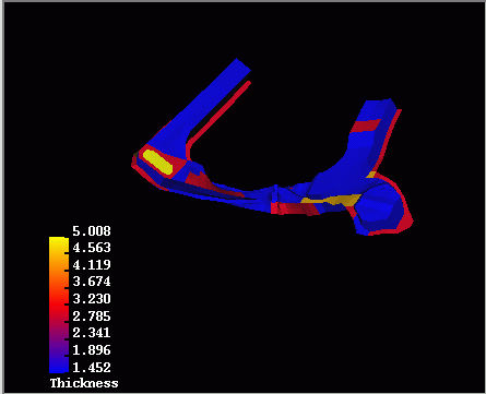
The model of the first example uses three kinds of elements: shells, bars and mesh-independent spotwelds. We plot in the three renderers the following magnitudes: velocity per node, shell thickness and axial bar force. Note the use of SplitUsg to realise the separation of elements of different dimensionality. Other modules that you may find useful when trying to visualise some parts of your model are AssembleUsg , CropUsg , PartSelect and ClipInterval . Below we produce the renderer output of the shell thickness.
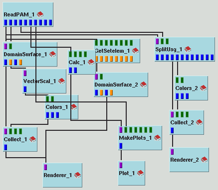
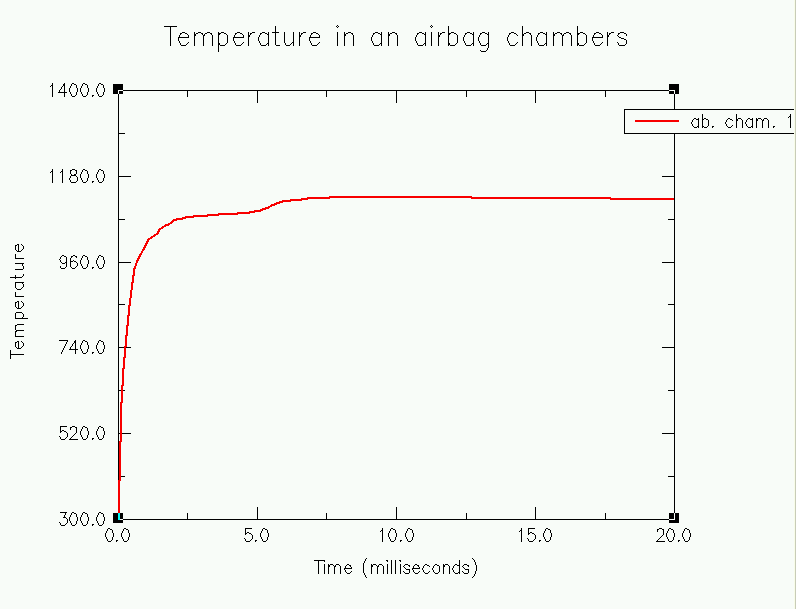
The model of the second example uses shells and tool elements. With this example we illustrate the visuallisation of non-local variables. We read file for the simulation of a multichambered airbag. We need in this case the modules MakePlots and Plot . The Plot output for the temperatures in one of the airbag chambers is produced below.
| Authors: Martin Aumüller, Ruth Lang, Daniela Rainer, Jürgen Schulze-Döbold, Andreas Werner, Peter Wolf, Uwe Wössner |
| Copyright © 1993-2022 HLRS, 2004-2014 RRZK, 2005-2014 Visenso |
COVISE Version 2021.12
|