• Starting COVISE
  • Introduction
  • Starting COVISE
  • The Mapeditor
  • Loading a Map

Starting COVISE

Introduction

After having read this chapter you will be familiar with:

• how to start COVISE
• the parts of the MapEditor
• how to load a map

COVISE is a toolkit to integrate several stages of a scientific or technical application such as simulations, reading of data, postprocessing and visualization. Each step is implemented as a module. Connecting these module forms a data flow network that can be executed. The user interacts with COVISE and its modules through a Motif based user interface.

Starting COVISE

After the installation the path to the covise executable is appended to the environment variable $PATH. To start COVISE type covise in a cshell or tcshell window.

This initiates the following processes: the controller which is responsible for message handling, the request broker, responsible for data handling, and the main user interface called MapEditor.

If the command covise is not found make sure you use a tcshell or a cshell. Otherwise have a look at the files README and INSTALL.TXT and check the environment variable COVISE_PATH. During the starting phase you might get the message Timelimit in accept exceeded Edit the file covise.config in the covise directory and increase the timelimit for your machine. You find more information about covise.config in Chapter 2 in the User's Guide.

COVISE can also be started with parameters. Typing covise help will show you the syntax.

The following 2 start options may be useful e.g. for demos with COVISE:

• -i start with MapEditor as icon
• -e execute immediately after loading

The Mapeditor

Figure: The Mapeditor

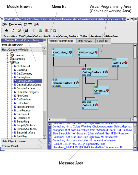
Figure 1.1: The Mapeditor

After the starting phase the MapEditor window (with Visual Programming as default) appears.

The MapEditor window consists of four main parts:

• the Menu Bar
• the Tool Bar
• one of three index cards according to the selected function
  • Visual Programming - default: to build a map
  • COVISE Objects - to look at the data structures involved
  • Control Panel - to modify parameters
• the Message Area

A Chat Line - used for communication together with the Message Area - appears in case of two or more users only.

The Visual Programming index card contains the Module Browser and the Visual Programming Area (canvas or working area). The Menu Bar contains an item File. You can have a new file, in which you create a data flow network, you can save a file or you can open a file that contains a saved session. Such a file is called a map. It contains a list of the modules in the map and information about the connections.

Creating a new module network (map) is discussed in chapter 3. In this chapter you learn how to load and execute a saved map. COVISE comes with some example maps and the maps described in this tutorial. They are located in the following directories:
$COVISEDIR/net/general/example
$COVISEDIR/net/general/tutorial

Loading a Map

Figure: Menu Item File

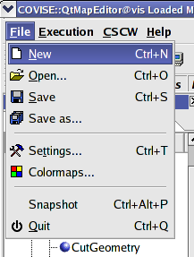
Figure 1.2: Menu Item File

The menu item File Open pops up a file browser (Figure 1.2). Select the file covise/net/tutorial/tutorial_pressure_1.net.

The loaded map appears in the working area. Each module is represented by an icon. A module has input data ports, represented by blue buttons on the top edge of the module icon and output data ports represented by blue buttons on the bottom of the icon. Green buttons mean optional data ports. Module icons are described in more detail in chapter 3.

When the Renderer module is started as part of the module network, its window is opened. Initially it contains only three coordinate axis. This is explained in more detail in chapter 2.

Now execute the network by selecting Execute in the Execution menu. One module icon after the other shows a red frame which indicates that it operates. Finally geometry objects appear in the render window (Figure 1.3).

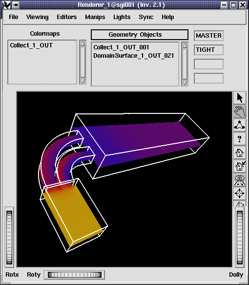
Figure: Geometry Objects in the Renderer

The left RWCovise module reads the grid file tiny_geo.covise. You select the grid via a file browser that pops up automatically.

Below RWCovise you find the module DomainSurface. Out of the whole 3D grid it extracts the outer surface or bounding lines of the grid. The DomainSurface module is directly connected to the Renderer module, which displays the results of DomainSurface. Figure 1.3 shows the content of the Renderer module window. The white lines are the bounding edges of the geometry. The displayed content is a flow channel with two inlets.

The second RWCovise module reads in the pressure distribution tiny_p.covise. CuttingSurface then computes a cutting plane in the pressure data. The module Colors converts the scalar data values to colors. The grid of the cutting plane and the colors are combined into a geometry object by the Collect module. Collect is directly connected to the Renderer, which displays the resulting colored plane.

Next