Overview | All Modules | Tutorial | User's Guide | Programming Guide

COVISE Online Documentation

Analysis of 3D Data

Analysis of 3D Data

Note for the experienced user:

This chapter has been reworked to demonstrate the new features for building maps quicker and easier. COVISE provides Complex Modules like TracerComp, CuttingSurfaceComp, or IsoSurfaceComp which include modules Colors, Collect etc.

For details please see Online Help, User's Guide, and Module Reference Guide.

Introduction

In this chapter you learn how to

visualize the computational grid
visualize vector data
visualize scalar data

This section gives a very short overview how to use COVISE modules for the analysis of simulation data.

In the example the bounding geometry is a channel with two inlets. The grid was created with PROSTAR, the pre- and postprocessing program for STAR and the simulation was performed with STAR. In a previous COVISE session the grid and the simulation result files have been converted to COVISE format, as this format allows very compact files and fast reading by COVISE.

In the directory covise/share/covise/example-data/tutorial you find the files

tiny_geo.covise
tiny_velocity.covise
tiny_p.covise
tiny_te.covise
tiny_vis.covise

tiny_geo.covise contains an unstructured grid while the other files contain data.

The following tutorial module pipelines (also called maps or nets) are located in the directory covise/net/general/tutorial/. In the next section only the most important module ports and parameters are explained. For detailed information about the modules a documentation in html format is available.

Visualizing the Computational Grid

Assuming we don't know what the files contain it may be useful to first make the simulation grid visible. The following modules have this or related functionality:

ShowGrid generates lines, points, hulls or bounding boxes for structured/rectilinear/uniform grids.

DomainSurface generates the outer surface of an unstructured grid.

SimplifySurface reduces the number of polygons representing a surface.

tutorial_grid_1.net

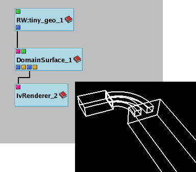
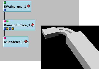
Start COVISE and open a new session. Choose the file tutorial_grid_1.net and execute the module network. Examining the module network, you see, that RWCovise is from the category IO-Module. It imports the data file tiny_geo.covise and generates an output data object containing an unstructured grid. The file name is specified as a file browser parameter.

The module DomainSurface from the category tools determines the outer surface of the grid or the edges of the outer surface. DomainSurface receives the unstructured grid as input data object. It produces polygons representing the outer surface which are available at the first output port.

This port is connected with the module Renderer which receives the poygons as input data objects. Figure 4.1 shows the map and the results displayed in the renderer window.

**Figure:** tutorial_grid_1

Figure 4.1: tutorial_grid_1

tutorial_grid_2.net

The disadvantage of the representation in Fig. 4.1 is that you can't see inside the channel.

Load the map tutorial_grid_2.net. The difference to the first map is that the third output port of DomainSurface is connected to the Renderer. This port outputs data objects which contain the edges of the outer surface.

**Figure:** tutorial_grid_2

Figure 4.2: tutorial_grid_2

tutorial_grid_3.net

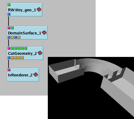
Another possibility to look inside the channel is to cut away parts of the geometry. This can be done by the module CutGeometry. Load the map tutorial_grid_3.net. The module CutGeometry cuts the geometry with a plane.

The plane is defined using the parameters scalar and vertex. Vertex defines the orientation of the plane and also the cutting direction. Scalar positions the plane along its normal direction. In this example vertex is [0.0 0.0 -0.1] and scalar is -0.12. This defines a plane which cuts away the upper surface of the channel.

**Figure:** tutorial_grid_3

Figure 4.3: tutorial_grid_3

tutorial_grid_4.net

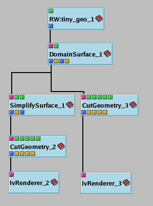
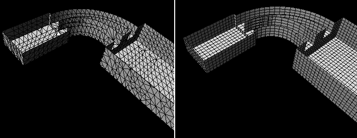
If a surface contains too many polygons, it can't be displayed with an acceptable frame rate (at least 12 frames per second).

For interactive handling it is necessary to reduce the number of polygons, which is done by the module SimplifySurface (see tutorial_grid_4.net).

**Figure:** tutorial_grid_4.net

Figure 4.4: tutorial_grid_4

**Figure:** Original and Reduced Surface

Figure 4.5: Original and Reduced Surface

Operating instructions for this example (to see how SimplifySurface works):

Use the "Discrete Mesh" representation (click with the right mouse button on the renderer window and choose DrawStyle > >DiscreteMesh.
Parameter "strategy": select "Vertex Removal" (click on the SimplifySurface icon to get the Module Information with the parameters)
Parameter "percent": specify the percentage of remaining triangles after SimplifySurface.

Visualizing Vector Data

Typical vector data resulting from a simulation is the velocity field. The following modules have to deal with vector data:

TracerComp

computes streamlines on unstructured grids
computes streamlines on structured grids
computes animated particle traces
contains additional functions to map output data to colors

(Historical Notes:
- In former versions of COVISE these functions had been implemented in 3 different tracers - TracerUsg, TracerStr, and TetraTrace
- If you specify e.g. animated particle traces, TracerComp, on top of standard Tracer, contains functions to show the particles as spheres and map data as colors on that spheres - no need for additional modules Sphere, Colors, Collect)

VectorField (explicitly used in tutorial_vel3.net only - otherwise contained, implicitly,in CuttingSurfaceComp)

computes small lines at each grid point. The direction of the lines represents the direction of the velocity vector and the size the amount of the velocity.

tutorial_vel_1_new.net

**Figure:** tutorial_vel_1_new

Figure 4.6: tutorial_vel_1_new

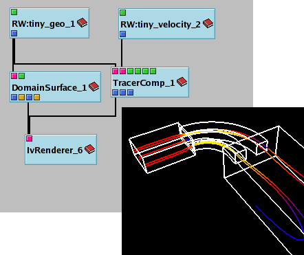
Load the map tutorial_vel_1_new.net. The second RWCovise module reads the data file tiny_velocity.covise which contains the velocity field.

The module TracerComp computes streamlines (Specify 'Streamlines' as parameter taskType in the Tracer). Its first input port receives the grid object and the second port the data object containing the velocity field.

The starting points of the streamlines and the number of streamlines are specified via module parameters.startpoint1 and startpoint2 define a line. no_of_startpoints defines how many streamlines start on this line. Usually it is difficult to determine the coordinates of the two points, if you don't know the size and position of the grid. In this example we choose [-0.4 0.5 0.02] for startpoint1 and [-0.4 0.3 0.02] for startpoint2 and draw 6 streamlines.

tutorial_vel_2_new.net

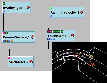
The map tutorial_vel_2_new.net shows an example of animated particle traces.

The layout of the map is the same as tutorial_vel_1_new.net, but you have to specify 'particle' in the parameter taskType in TracerComp. i The output of TracerComp contains sets of points where each set represents the position of the particles at a certain timestep, together with velocity data attached to the points. TracerComp integrates the function to make particles more visible by displaying small spheres instead of points (specify radius as parameter) and to map output data to colors.

As soon as the pipeline is executed, the geometry is displayed in the renderer window. In addition, the renderer contains a slider for selecting the timesteps of the animation. For a continuous animation press the play button.

**Figure:** tutorial_vel_2_new

Figure 4.7: tutorial_vel_2_new

tutorial_vel_3.net / tutorial_vel_4.net

The map tutorial_vel_3.net is an 'old-fashioned' map - have a look at it for information only and don't use it as an example; it shows a flow visualization with small lines attached to the grid points which depict the magnitude and the direction of the respective velocities.

The module VectorField needs the grid and the velocity data as input data objects and computes lines and data attached to the lines as output objects. The data are mapped to colors using Colors and Collect.

**Figure:** tutorial_vel_4_new

Figure 4.8: tutorial_vel_4_new

Displaying vector dashes at all grid points is not very useful. Instead a CuttingSurfaceComp module can extract a 2D subset of the grid of which the grid points are then used to attach the vector dashes (see tutorial_vel_4.net). Note that the data attached to the cutting plane is determined by interpolating in the original grid. Since displaying vector data as colored arrows on a cutting surface is a frequently used operation, this function has been integrated into CuttingSurfaceComp (see Fig. 4.8) and is automatically activated in case of vector data! Colors is used to select a colormap for the colors on the vector dashes.

Visualizing Scalar Data

Typical scalar data resulting from a simulation are e.g. pressure or temperature. Modules for visualizing scalar data are:

CuttingSurfaceComp computes a cutting plane, cylinder or sphere in unstructured grids. In addition, it can map scalar data to colors. IsoSurfaceComp computes a surface connecting all points in space, which have the same scalar value. In addition, it can map scalar data to colors. Colors is used in this example to select a colormap (including minimum, maximum, annotation)

tutorial_pressure_1_new.net

**Figure:** tutorial_pressure_1_new

Figure 4.9: tutorial_pressure_1_new

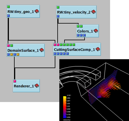
Load the map tutorial_pressure_1_new.net. Additional to the RWCovise module which reads the grid we have a second RWCovise module which reads the pressure data file tiny_p.covise.

CuttingSurfaceComp from the category filter then extracts a surface (plane, cylinder, sphere). It needs the grid object and the data object containing scalar data as input and creates polygons or tristrips which form the cuttingsurface and data on the surface as output objects. In addition, the data are mapped to colors and combined into a geometry object together with the polygons/tristrips.

Using the parameter option you define the shape of the surface. Map the parameter to the ControlPanel by clicking on the button in front of the parameter. Now you can see that you have the options plane, cylinder and sphere. Using the parameters vertex and scalar you specify the orientation and position of the surface.

For a plane the parameter vector is the normal of the plane and the scalar is the distance of the plane from the origin. In this example the normal of the plane is (0 0 1) and the distance from the origin is 0.05.

A scalar parameter such as the distance is defined using three numbers: minimum, maximum and current value. Map the parameter distance to the ControlPanel. The default interactor in the control panel is a VCR type player. You can increase or decrease the distance via the player buttons applying a certain increment which is specified in an extra field. Modify the distance parameter to get an overview of the pressure distribution in the channel.

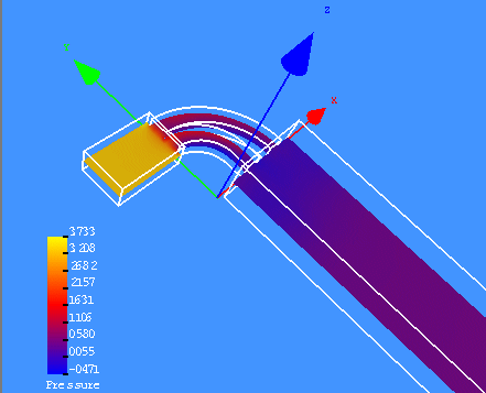
In the render window you can also see a color bar. Color bars are produced by the modules Colors and ColorEdit (explicitly or implicitly, if the function of Colors is integrated e.g. in the complex module CuttingSurfaceComp). They are only displayed in the render window if they are selected there. Click on the name of the data object to pop it up and click again to hide the colorbar.

Note: The module Colors_2 is used to select the colormap, the minimum and maximum values, and the annotation, e. g. "Pressure" (default: Colors).

**Figure:** tutorial_pressure_1_new: Results in the Renderer

Figure 4.10: tutorial_pressure_1_new: Results in the Renderer

tutorial_pressure_2_new.net

**Figure:** tutorial_pressure_2_new

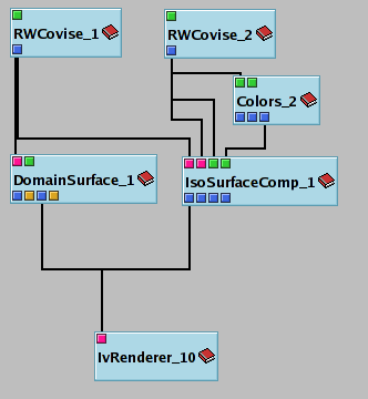
Figure 4.11: tutorial_pressure_2_new

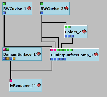
Another method to visualize scalar data are isosurfaces. An isosurface is a surface consisting of points in space, where the scalar data has the isovalue. Load the map tutorial_pressure_2.net and execute it. The blue surface connects all grid points where the pressure has the value 0.05.

Have a look at the map in the MapEditor window. Again the first RWCovise reads the grid while the second one reads the pressure data.

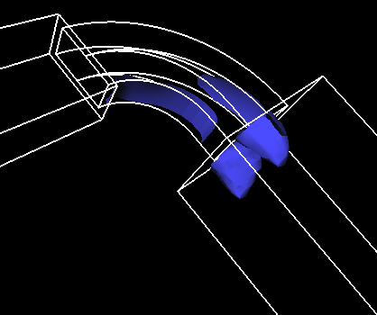
**Figure:** tutorial_pressure_2_new: Results in the Renderer

Figure 4.12: tutorial_pressure_2_new: Results in the Renderer

IsoSurfaceComp needs the grid and the scalar data as input objects. The resulting polygons or tristrips are provided at the first output port and the data on the surface at the second port. The isovalue is defined using the input parameter isovalue. The parameter gennormals enables the generation of normals at each polygon vertex.

The normals are available at the third output port.. The normals are used for the computation of the surface lighting. If you do not provide normals for a surface the renderer computes one normal per polygon face. Normals per vertex result in smoother surfaces than normals per face.

Note: Like CuttingSurfaceComp in tutorial_pressure_1_new.net, IsoSurfaceComp maps the data to colors. The Module Colors_2 is used to select the colormap, the minimum and maximum values, and the annotation, e. g. "Pressure" (default: Colors).

Summary (Example)

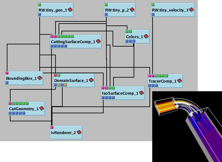
channel_new.net

The example channel_new.net below combines some of the features shown before in one map. In addition, it shows how to get the size of your geometry object using the BoundingBox module.

**Figure:** channel_new

Figure 4.13: channel_new

Authors: Martin Aumüller, Ruth Lang, Daniela Rainer, Jürgen Schulze-Döbold, Andreas Werner, Peter Wolf, Uwe Wössner

COVISE Version 2021.12