| Overview | All Modules | Tutorial | User's Guide | Programming Guide |
Module category: Obsolete
TracerUsg performs computation of particle tracks inside unstructured grids or blocks of unstructured grids. It uses a Runge-Kutta 2nd- or 4th-order numerical integration method. It may handle also time steps. In this latter case the output may not be the physical trace of particles in the fluid, but it may be helpful for the sake visulisation.
Note:
Module obsolete - kept for compatibility with 5.1 only, but support discontinued - use Tracer (new with 5.2) instead!
| Name | Type | Description |
| no_startp | Slider | number of particles to trace. |
| startpoint1 | Vector | Start point of a line, if startStyle is line, or a corner point of a rectangle of stating points, if startStyle is plane. |
| startpoint2 | Vector | End point of a line, if startStyle is line, or the opposite corner point of a rectangle of stating points, if startStyle is plane. |
| direction | Vector | Vector describing the direction of one side of the rectangle of initial points (only relevant if startStyle is plane). |
| amesh_path | Browser | File containing a two-column ASCII list of block number pairs, which indicate the neighbourhood of the grid blocks. The functionality associated to this parameter is still in construction, so you need not worry about it. |
| option | Choice | Order of the Runge-Kutta integrator. |
| stp_control | Choice | Step control method:
“position” computes the time step using the velocity and the cell size at the current position, 5 < angle < 12 or 2 < angle < 6 compute the step width using the angle between two velocity vectors, in a way that the time step is increased or decreased in order to try to remain in the pertinent interval. The first choice is by far safer than the other two options. |
| tdirection | Choice | You may choose among:
|
| reduce | Choice | Reduction of the number of points in the streamline. “Off” disables reduction, “3deg” and “5deg” use the angle between the velocity vectors for reducing the number of points. Reduction of points also includes reduction of corresponding data values. “3deg” and “5deg” therefore don't display data on the streamlines as accurately as in the “Off” case, especially where the reduction may be very strong, that is to say, where the lines are almost straight. |
| whatout | Choice | Select what data will be available at the second output port. You have the choice between the velocity magnitude (“mag”), the x, y, or z component (“v_x” “v_y” “v_z”), or the module may assign a fixed number to a line (“number”). When mapping the data on the line to colours and you have choosen “number” each line has a different color. |
| trace_eps | Scalar | Relative tolerance for deciding if a point is in a cell. |
| trace_len | Scalar | The integration for a line is interrupted when it attains this length. |
| startStyle | Choice | how should the particles
starting positions be arranged:
|
| MaxPoints | Scalar | It limits the maximum number of points in the
output lines.
Note: If velocity goes to 0, it makes no sense to increase "MaxPoints" - ignore the corresponding message! |
| MaxSearchFactor | Scalar | It sets a limit to the maximum size of a box about a possible starting point, in which the starting cell is looked for. For grids in which the element sizes do not vary very wildly, the default value will usually be big enough; but it may eventually happen that you have to increase this number for this module to be able the find the cell containing some point. The greater the value of this parameter is set, the slower this module will be. In this sense, the default value is rather conservative. But if the integration has been interrupted by the module and this was not correct, this may be a sign that a greater value of this parameter is required. On other occasions this may be an indication that a wall has been incorrectly detected (this is only relevant for grid sets), then you have to modify parameter Speed_thres. |
| Speed_thres | Scalar | It sets a threshold for wall detection. When the trajectory crosses the border between two blocks (two grids that are elements in a set), the module works out the velocity on both sides and their difference. If the length of the difference is less than this parameter multiplied by the maximum of the magnitudes of both velocities, then the module assumes that this interface is not a wall. Otherwise it interpretes that a wall has been found and the integration is interrupted. If you want to deactivate this feature, then introduce a negative number. This has in general the same effect as if a huge positive number were introduced. |
| Connectivity | Boolean | If TRUE the reader assumes that the grid connectivity is correct in the sense that it may be used in order to determine the neighbour cells of a given cell. TRUE is the default value because then the performance is better. Nevertheless, it may happen that in your grid the connectivity may not be relied upon for this purpose, for instance if some parts of the grid have been refined in a such a way that some nodes are lying between two elements but they only belong to the element of the refined region. Then you have to set this parameter to FALSE, otherwise the trace integration is interrupted when this unconnected interface is reached. |
The third input port is associated to the functionality of parameter amesh_path, which is in construction, so you need not worry about it.
| Name | Type | Description |
| requiredmeshIn | DO_UnstructuredGrid | Input mesh |
| requireddataIn | DO_Vec3 DO_Vec3 | velocity on the grid nodes |
| optionalcellTypeIn | DO_IntArr | --- |
|
|
| Name | Type | Description |
| outputlines | DO_Lines | Streamlines |
| outputdataOut | DO_Float | the output data (as specified by parameter whatout mapped on the traces |
| outputvelocOut | DO_Vec3 | the velocity mapped on the traces |
|
|
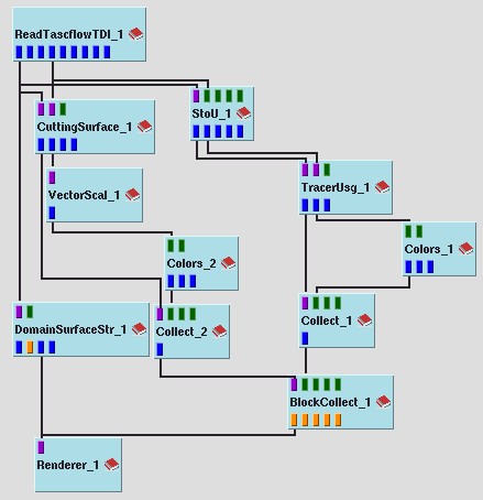
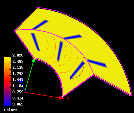
In this example we integrate the velocity field in a domain for 6 different initial conditions. This domain is defined by a set with two structured grids. A StoU module is used to get a set of unstructured grids. One might use in this case TracerStr without any need for StoU, but we use this procedure for the sake of illustrating TracerUsg. Observe in the renderer images below that in the domain there are some regions, which coincide with blades in a rotor, with null velocity. This regions are shown in blue. The colours on the line map the magnitude of the velocity.
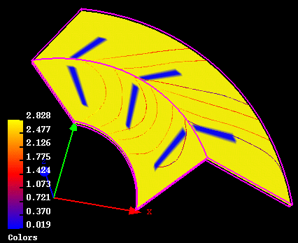
The output is produced below for two cases. With the default value for wall detection (parameter Speed_thres), the trajectories stop when they arrive at the border between the grids, because a severe discontinuity of the velocity field is detected. The output (Speed_thres=0) may be seen in the first image. The second image (Speed_thres=-1) shows what happens if we deactivate this feature by introducing a negative value for parameter Speed_thres. A similar effect could be achieved by introducing a big enough positive number. The deactivation of this feature may be useful if we know that the discontinuity appears because the velocity in both domains is measured in different reference systems. The trajectories are then continued in the second grid.
| Authors: Martin Aumüller, Ruth Lang, Daniela Rainer, Jürgen Schulze-Döbold, Andreas Werner, Peter Wolf, Uwe Wössner |
| Copyright © 1993-2022 HLRS, 2004-2014 RRZK, 2005-2014 Visenso |
COVISE Version 2021.12
|