| Overview | All Modules | Tutorial | User's Guide | Programming Guide |
Module category: Mapper
The TracerComp module performs particle tracing within vector fields. It can either show Floating Particles or connect these to Streamlines, Streaklines, and Pathlines, which are different for transient data.
The key difference with respect to the normal Tracer module, is that TracerComp relieves you from the burden of connecting the output with Colors, Collect and Sphere modules. You may directly connect the first output port with the renderer.
The data can be given on structured and unstructured grids and also on Polygons. If the data is given on Polygons, the traces are bound to the polygons even if the velocities have components pointing out of it. The Polygons do not have to be planar.
Starting points can be given equally spaced on either a line or a rectangular area in 3D space, either by numerical input or interactive by VR manipulators in COVER.
TracerComp is available for all supported platforms.
| Name | Type | Description |
|
no_startp | Slider | Starting point selection: see below |
| startpoint1 | Vector | Starting point selection: see below |
| startpoint2 | Vector | Starting point selection: see below |
| direction | Vector | Starting plane direction: see below |
| Displacement | Vector | Constant offset added to all lines |
| tdirection | Choice | Trace direction: Forward, Backward, Both |
| whatout | Choice | mag / v_x v_y v_z / time |
| taskType | Choice | select between Moving Points, Stream-, Streak- or Pathlines |
| startStyle | Choice | line, plane or free |
| trace_eps | Scalar | Finetuning parameter for Trace integration (Maximum permitted relative error per integration step. This parameter is involved in the control of the integration step.) |
| trace_abs | Scalar | Finetuning parameter for Trace integration (Maximum permitted absolute error per integration step. This parameter is involved in the control of the integration step.) |
| grid_tol | Scalar | Tolerance value for grids with gaps |
| trace_len | Scalar | Finetuning parameter for Trace integration (Maximum length for streamlines.) |
|
min_vel | Scalar | Finetuning parameter for Trace integration (Minimum velocity for streamlines. If along the integration of a streamline, the velocity is found to be smaller than this value, the integration is interrupted.) |
| MaxPoints | Scalar | Number of Steps for Moving Points |
| stepDuration | Scalar | Time stepping used in transient traces and for moving points |
| NoCycles | Scalar | For transient cases: repeat input steps |
| NoInterpolation | Boolean | Finetuning parameter for Trace integration (This parameter is only relevant for moving points or pathlines with static data. The default value is false. This means that the last point of the pathlines, if you have chosen this option in the parameter "taskType", or the points you see, in the case of moving points, have been evaluated by an interpolation between two consecutive points of a calculated streamline. This is faster than the true option, especially if stepDuration is very small. In the case true, the step control of the integration is disturbed in a way that it is forced to calculate values for the times we need for output. The true case is only recommended for rather large values of the stepDuration parameter, otherwise the performance penalty may be important. In most cases the default false value is preferable.) |
| ThrowNewParticles | Boolean | Throw new particles in multiple timesteps |
| ParticlesReleaseRate | Scalar | Frequency at which new particles are released |
| divideCell | Scalar | Finetuning parameter for Trace integration (This parameters sets the integration step when the integrator has detected that the particle is not far from a wall (the border of a grid), so that the distance covered by the particle in a time step is approximately the value of this parameter multiplied by a cell typical distance. This number should always be positive.) |
| maxOutOfDomain | Scalar | Follow particles out of cell - increase if grid has gaps the particles should fly through |
| NoWThreads | Scalar | Multi-Threading: 0 means single-thread |
| SearchLevel | Scalar | Search depth for polygon tracing starting points. Increase when staring points are not found |
| SkipInitialSteps | Scalar | This is relevant on dynamic data sets for pathlines, moving points and streaklines. You may control with this parameter the initial step at which particles are released. |
| color | String | The color of the streamlines. |
| SphereRadius | Scalar | In case that you are producing moving points, you may directly visualise them as spheres by directly connecting the first output port with the renderer. This parameter controls the sphere size. |
| FreeStartPoints | String | List of points. E.g. "[1., 2., 3.][0., 0., 0.]" |
| Min/Max | Vector | Minimum and Maximum value |
| autoScales | Boolean | Automatically adjust Min and Max |
| Name | Type | Description |
| requiredmeshIn | UnstructuredGrid UniformGrid RectilinearGrid StructuredGrid Polygons | Input mesh |
| requiredveloIn | Vec3 Vec3 | velocity on the grid nodes |
| optionalpointsIn | Points | If a Points object is given at the "pointsIn" port, it overrides the starting point parameters and the points in the data objects are used instead. This way you may achieve an arbitrary spacial distribution of initial points. |
| optionalocttreesIn | OctTree OctTreeP | The tracer builds internally an octree for the input grids upon the first execution. In some cases, for instance, if you are using several tracer modules for the same data set, or if you want to use non-default values for the parameters involved in the octree build-up, you may want to use construct these octrees elsewhere, for instance using the MakeOctTree module, and hand them down to the tracer module. |
| optionalcolorMapIn | ColorMap | You may have the module use a given colormap using this module. Otherwise the module will internally generate a colormap based on the scalar magnitude being produced for the output. |
| Name | Type | Description |
| outputgeometry | Geometry | You may connect this port directly with the renderer. |
| outputlines | Lines Points TriangleStrips | Streamlines |
| outputdataOut | Float | the output data (as specified by parameter whatout mapped on the traces |
|
|
Moving Points
A cloud of points is emitted into the flow at given positions and then advanced according to the given vector field. If the field is transient, the number of steps is the number of timesteps in the given field; otherwise it can be selected by the "MaxPoints" parameter.
The length of the time interval for each step can be chosen with the "stepDuration" parameter unless a REALTIME attribute is attached to a transient input data set, which overrides user settings.
Streamlines
Streamlines are integration lines across the vector field. From a given starting point, the particle path is integrated in the direction given by the "tdirection" parameter. Streamlines are calculated independently for each timestep in transient fields.
Streamlines are limited by the "trace_len" parameter, which is a limit for the maximum length of the line in model coordinates.
Streaklines
Streaklines require transient data. They imitate a smoke probe of a wind channel: At every time step, new particles are emitted from the starting point and connected by lines.
If the data set does not contain a REALTIME attribute (currently only supported by the StarCD reader), the time spacing of the transient data must be constant and manually be correctly entered in the "stepDuration" field to get a correct streakline.
Pathlines
The Pathlines otion is available for both static and dynamic data sets. In this case the path of a particle is traced and shown. For moving grids, this may even create lines outside the geometry in later time-steps. As for the Streaklines, the time stepping must be set correctly.
All traces running on transient data may emit partices multiple times by the "ThrowNewParticles" switch. In this case, the "ParticlesReleaseRate" parameter defines the release frequency.
With the "NoCycles" parameter the data set can be interpreted as a cyclic set of data and repeated multiple times.
Two different kinds of starting points can be selected with the "startStyle" choice:
If a Points object is given at the "pointsIn" port, it overrides the starting point parameters and the points in the data objects are used instead.
The "displacement" parameter allows to offset the trace by a constant value - this may be used especially with traces along surfaces to make them visible on hardware with z-Buffer.
The particle tracer uses Octrees to accelerate the tracing of unstructured grids. These can be supplied by an input object, otherwise they are created internally.
When using multiple Tracers on the same grid it is more efficient to create the octree for the grid once by the "MakeOctree" module and supply it to all Tracers.
When a trace is interrupted before you expect it, and "taskType" is "Streamlines", you should consider either of the following reasons:
Trace terminates at grid anomalies
The tracer stops integration at the boundaries of the grid. Any gap in the meshing may appear as a boundary and thus stop the tracing. There are several parameters to overcome these problems:
This parameters sets the integration step when the integrator has detected that the particle is not far from a wall (the border of a grid), so that the distance covered by the particle in a time step is approximately the value of this parameter multiplied by a cell typical distance. This number should always be positive.
When the integration goes beyond a grid, integration is interrupted if no other grid is found to pursue the integration, but this is not done immediately. Integration is pursued for a short distance even the particle is out of the domain, this distance is given by the value of this parameter relative to a typical cell length. This value should be at least twice the value of "divideCell".
The most basic parameter is "taskType", which fixes the kind of task to be done. According to this choice, irrelevant parameters are disabled, so that you may concentrate on those parameter that might be relevant for your task.
When a trajectory is interrupted before you expect it to occur, and "taskType" is "Streamlines", you should consider either of the following reasons:
With the animation options of the "taskType" parameter "Moving points", "Pathlines" or "Streaklines", integration is pursued up to the required time or until the integration gets out of the domain. "trace_len" and "min_vel" are irrelevant in this case. Parameter "MaxPoints" is still relevant, but it has a different meaning, which has nothing to do with the interruption of a trajectory. In these cases "MaxPoints" is only relevant for static data, and it determines the number of time steps of your animation. On the other hand, parameter "NoCycles" is only relevant for dynamic data, as explained in the section devoted to parameters. Do not change its value unless it is meaningful, because the computation time will increase accordingly, or the integrator may have numerical problems if you do not have a whole cycle.
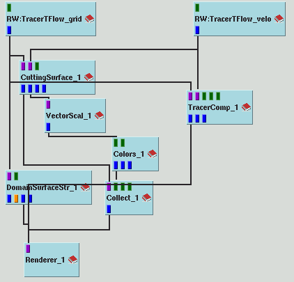
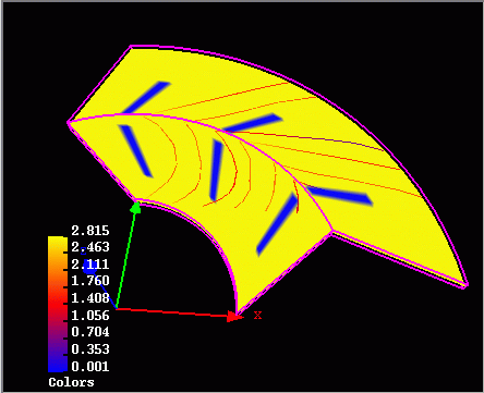
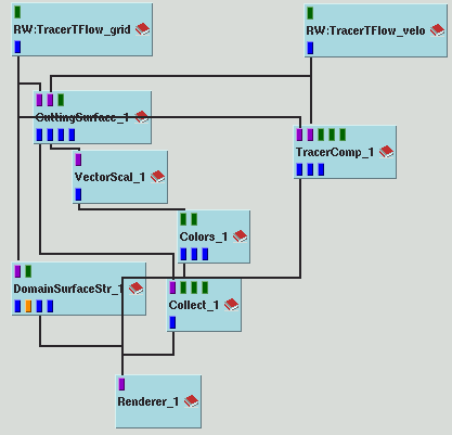
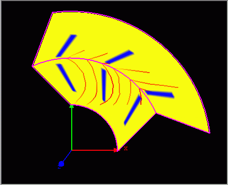
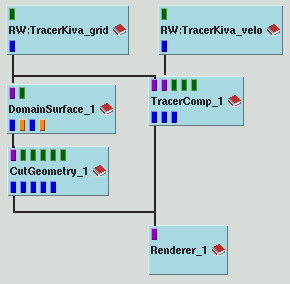
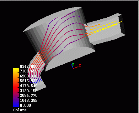
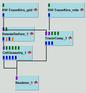
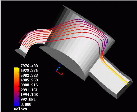
In the first example we integrate the velocity field in a domain for 6 different initial conditions. This domain is defined by a set with two structured grids. Observe in the renderer image below that in the domain there are some regions, which coincide with the blades in a rotor, with null velocity. This regions are shown in blue. The colours on the line map the magnitude of the velocity.
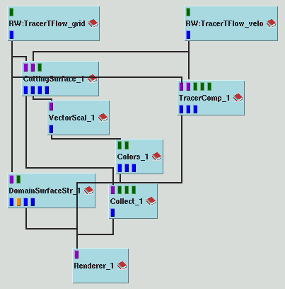
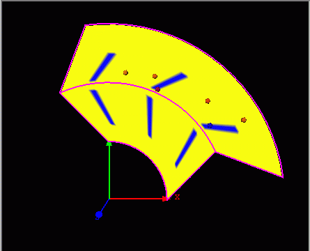
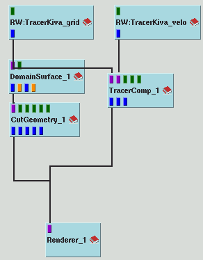
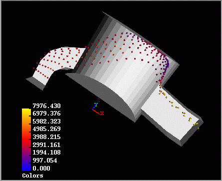
The second example produces an animation with 250 time steps of moving points for the same input static data as before. A snapshot of the animation is shown.
The third net file produces an animation with 250 time steps of pathlines for the same input static data as before. A snapshot of the animation is shown.
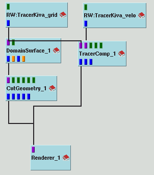
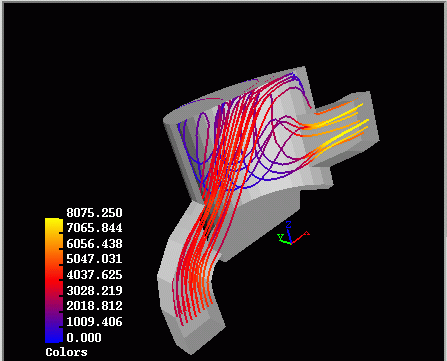
In the 4th example we have a dynamical input grid. Streamlines do not represent the physical particle motion but may be useful for visualisation, as here. The output for the last time step is shown below. There are no streamlines for the first time step, because at that instant of time the velocity is null on the domain.
In the 5th example we integrate the physical trajectory upon the assumption of some value for the real time between time steps (see parameter stepDuration). The last time step of the output is shown. Observe that it is different from the previous renderer image for streamlines.
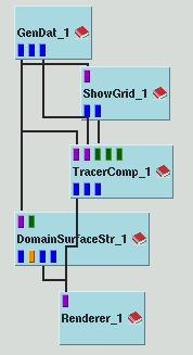
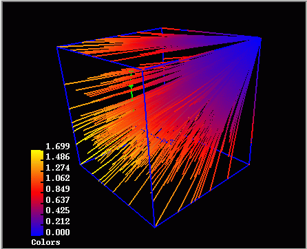
In the 6th example we integrate streamlines on a static domain. Now we are using the third input port for the initial points. We generate a Points object with the ShowGrid module. The output is shown below.
In the 7th example we integrate streaklines for dynamic data. Note that we have to set a high enough particle release rate in order to get beautiful results. The output is shown below for the last time step. Note that the output is not the same as that for pathlines (example 5).
In the 8th example we integrate moving points for dynamic data. The output is shown below for the last time step. Particles are released at the same rate used in example 7 for streaklines. The output of example 7 may be obtained by joining the pertinent points of this 8th example.
|
| Authors: Martin Aumüller, Ruth Lang, Daniela Rainer, Jürgen Schulze-Döbold, Andreas Werner, Peter Wolf, Uwe Wössner |
| Copyright © 1993-2022 HLRS, 2004-2014 RRZK, 2005-2014 Visenso |
COVISE Version 2021.12
|