| Overview | All Modules | Tutorial | User's Guide | Programming Guide |
Module category: Interpolator
Sample resamples point-based, uniform or unstructured data to a uniform grid.
Data cells in the destination uniform grid that are not intersected by the input data are either set to a certain value or the maximum float value (see parameter outside). The module Colors computes a transparent color for MAX_FLT data, so that those parts appear transparent in the COVER. If you use the Inventor Renderer set the value fill_value to a value which is in the range of your data set. In this case you will have to activate one of the `blended' modes of the Inventor Renderer under the `Viewing' item of the menu bar.
A uniform grid and colors on the uniform grid can also be seen as a 3D texture. If you cut a plane out of the 3D texture you get a 2D texture (an image). Mapping this texture on a plane gives similar information as a cuttingsurface through the 3D grid with data mapped on the surface as colors. Volume rendering can be used to display the data on all the uniform grid at once.
3D textures are supported by Octane and Onyx systems as well as Nvidia Geforce/Quadro 4 or newer and are computed by the graphics hardware and are thus very fast.
Sample has been tested on SGI platforms.
| Name | Type | Description |
| outside | Choice | Select if MAX_FLT or a number should be used to fill the parts of the uniform grid which are not intersected by the input data. The module Colors maps MAX_FLT to fully transparent in the COVER. |
| fill_value | Scalar | This parameter is enabled only if parameter outside is set to number. |
| algorithm | Choice | You may select one algorithm out of 4 available choices. They have been ordered according to their rapidity. The first choice being the fastest; and the last one, the slowest. We reserve a subsection below for a discussion of these algorithms. |
| point_sampling | Choice | Either the number of points (or the sum of the corresponding data values if the data input port is connected) or the logarithm thereof is computed as the value of a cell. This can be normalized so that the value does not change in magnitude when another sampling accuracy (size of the output grid) is chosen. |
| isize | Choice | Dimension of the uniform grid in i-direction. You can select between predefined sizes or you select user defined and enter the size with the parameter user_defined_isize. The predefined sizes are the sizes needed for the CuttingPlane3DTex plugin. |
| user_defined_isize | Scalar | This parameter is enabled only if isize is set to user_defined. |
| jsize | Choice | Dimension of the uniform grid in j-direction. See parameter isize. |
| user_defined_jsize | Scalar | See parameter isize. |
| ksize | Choice | Dimension of the uniform grid in k-direction. See parameter isize. |
| user_defined_ksize | Scalar | See parameter ksize. |
| bounding_box | Choice | If you select on of the automatic options, the module creates a uniform grid spanning the bounding box of the input grid. This bounding box can be calculated for each timestep or for all timesteps. By choosing the option manual, you have to introduce two corner points of the bounding box fixing the dimension of the uniform output grid. |
| P1_bounds | Vector | Coordinates of the first corner point of the bounding box if you choose manual in parameter bounding_box. |
| P2_bounds | Vector | Coordinates of the second corner point of the bounding box if you choose manual in parameter bounding_box. |
| eps | Scalar | A small value which can be used to avoid holes inside the data in the case of the slowest algorithm. |
|
|
| Name | Type | Description |
| requiredGridIn | UniformGrid UnstructuredGrid Points | The uniform or unstructured grid or points. |
| optionalDataIn | Float Vec3 Float Vec3 | Scalar or vector data on the uniform or unstructured grid or at the points. The data has to be vertex-based. If you have cell-based data use the module CellToVert to convert the data. |
| optionalReferenceGridIn | UniformGrid | Uniform grid to be used as destination grid, the parameters for defining the destination grid are ignored if this port is connected. |
|
|
| Name | Type | Description |
| outputGridOut | UniformGrid | The sampled grid. |
| dependDataOut | Float Vec3 | Scalar or vector data on the uniform grid. |
|
|
traverse all unstr grid nodes
{
   find the closest node of the uniform grid

   add the inverse of the distance to an accumulator
         for this node of the uniform grid.

   calculate a value using the product of the value
         at the input-grid node and the inverse of the distance.
}

traverse all unigrid nodes
{
   use the accumulator for this node in order
         to obtain the correct value.
}
This is the fastest one, but if the input grid is coarser than the output uniform grid in some regions, holes may appear; that is to say, some nodes of the uniform grid that are within the domain of some element of the input grid, have been given a value as if they were beyond the domain of the input grid. Holes may be apparent, but sometimes not (for instance CuttingSurface could smear out this holes producing false results which are not apparent at first sight). This latter situation may lead to confusion, that is why this algorithm has to be used with caution.
traverse all unstr grid elements
{
   calculate the largest box of nodes of the uniform grid
           that is fully contained in this element.

   for all nodes in this box
   {
      for all nodes of this element of the unstr grid
      {
         add the inverse of the distance to an accumulator
            for this node of the box.

         calculate a value using the product of the value
            at the unstr-grid node and the inverse of the distance.
      }
   }
}
traverse all unigrid nodes
{
   use the accumulator for this node in order
         to obtain the correct value.
}
This is the default algorithm and it is heartily recommended in most situations. Holes are avoided. One feature of this algorithm is that the sharpness of geometric features are better preserved than with the third algorithm. Sometimes this may lead to some features being shrunk. For instance, if you have a model with some pipe-like structures communicating two vessels, the pipe thickness that you see may be reduced. If this is really a problem for you, then you may use the third algorithm, but then be aware that the calculation may take longer and the geometric details may be blurred, which you will most likely not prefer.
traverse all unstr grid elements
{
   calculate the smallest box of nodes of the uniform grid
           that fully contains this element.

   for all nodes in this box
   {
      for all nodes of this element of the unstr grid
      {
         add the inverse of the distance to an accumulator
            for this node of the box.

         calculate a value using the product of the value
            at the unstr-grid node and the inverse of the distance.
      }
   }
}
traverse all unigrid nodes
{
   use the accumulator for this node in order
         to obtain the correct value.
}
Although this algorithm closely resembles the second one, it is in general significantly slower. Geometric features are now not shrunk, but rather expanded and blurred.
traverse all unstr grid elements
{
   find min and max unigrid indices by rounding to
   next smaller grid point

   for each unigrid point between min and max unigrid index
   {
      test if point is inside element

      if inside
      {
         interpolate using the form functions from the
            finite element theory for this element.
      }
   }
 }
For the test if a point is in a cell the cell is decomposed into tetrahedera. For each tetrahedron it is tested if point is inside the tetrahedron (The barycentric coordinates of the point in relation to the tetrahedron are computed. If the barycentric coordinates are between 0 and 1 the point is in.) This leads to the following problems:
In case that holes appear you may give parameter eps a small positive value. Then the condition for the point to be inside the element is that the barycentric coordinates are between 0-eps and 1+eps.
Holes seldom appear with this algorithm, and if they do, it is most of the times near the borders of the grid. Nevertheless, on some occasions holes have been seen in the interior of the model. In this situations you may have to use parameter eps to prevent holes from happening.
Apart from these occasional problems, the values obtained with this algorithm are most accurate, but the price to pay for this accuracy is a rather long execution time.
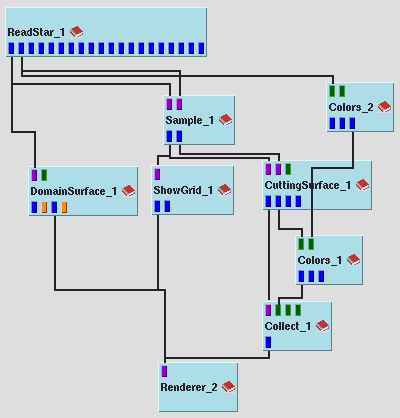
The first input for Sample is an unstructured grid and the second input are vertex-based data on unstructured grids. In the example the computational grid is a channel with two inlets and the data is the turbulent energy.
The dimension of the sampled grid was 30x30x30 and the fill value of Sample was set to 0.0.
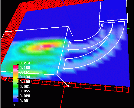
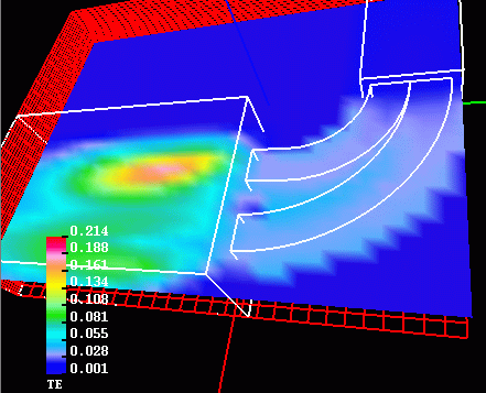
We produce two images corresponding to the second and third algorithms respectively. We want to illustrate how one produces sharper geometrical details and the other produces an expansion and blurring of them. This is clearly seen for the two inlets of the structure.
| Authors: Martin Aumüller, Ruth Lang, Daniela Rainer, Jürgen Schulze-Döbold, Andreas Werner, Peter Wolf, Uwe Wössner |
| Copyright © 1993-2022 HLRS, 2004-2014 RRZK, 2005-2014 Visenso |
COVISE Version 2021.12
|