Module category: Filter

• CuttingLine
  • Parameters
  • Input Ports
  • Output Ports
  • Examples

CuttingLine

CuttingLine extracts a line from a structured data set and creates an 2D object. In general you will use the module Plot to display this object.

Parameters

Name	Type	Description
cutting_direction	Choice	You can choose the direction which should be variable. If you imagine a 2D-plot this corresponds to the values used on the x-axis. Therefore the data value at this point is displayed along the y-axis of the plot. More over you can enter a range of indexes on the chosen axis. The range begins at the corresponding index parameter and ends with the maximum index in this direction.
i_index	Scalar	Constant index in x- direction or start of index range if cut along i is chosen.
j_index	Scalar	Constant index in y- direction or start of index range if cut along j is chosen.
k_index	Scalar	Constant index in z- direction or start of index range if cut along k is chosen.

Input Ports

Name	Type	Description
requiredmeshIn	UniformGrid RectilinearGrid StructuredGrid	Structured grid.
requireddataIn	Float Vec3	Data on structured grid points. The use of vector data is not implemented yet.

Output Ports

Name	Type	Description
outputdataOut	Unstructured_S2D_Data	Data on cutting line.

Examples

Figure: covise/net/examples/CuttingLine.net

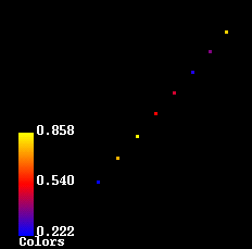
With the module GenDat we create a simple structured data set. On the one hand we display the data values on a cutting line by colors. Therefore we use the module FilterCrop to extract one line out of the structured grid. You can see the resulting points and their data values visualised by colors in the first image. To reproduce the same image as shown in the example docu, use the draw option points in the renderer or insert the module 'Sphere' between ShowGrid and Collect to make points visible. More over go to the Colormaps window in the information area of the renderer and click on Collect_1_OUT to get the colormap displayed in your renderer window to see the scaling.
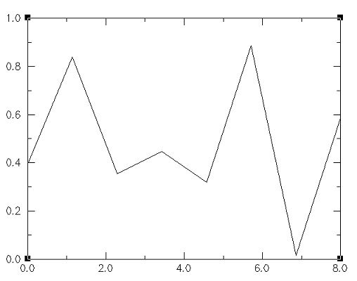
One the other hand we use the module CuttingLine to dislay the same values as a 2D plot. The result is shown in the second image. On the x-axis of the plot you can find the used index range, here from zero to eight.

Figure: Data values visualised by colors

Figure: Data values displayed as 2D- Plot