README

Exercise 4: Strided Data Access Patterns (and how to find them)

This exercise uses a simple implementation of a yAx kernel to show how difficult strided data access patterns can be to spot in code, and demonstrates how to use omniperf to begin to diagnose them.

Note: This exercise was tested on a system with MI210s, on omniperf version 2.0.0 and ROCm 6.0.2 Omniperf 2.0.0 is incompatible with ROCm versions lesser than 6.0.0

Background: Acronyms and terms used in this exercise

L1: Level 1 Cache, the first level cache local to the Compute Unit (CU). If requested data is not found in the L1, the request goes to the L2
L2: Level 2 Cache, the second level cache, which is shared by all Compute Units (CUs) on a GPU. If requested data is not found in the L2, the request goes to HBM
HBM: High Bandwidth Memory is globally accessible from the GPU, and is a level of memory above the L2 cache
CU: The Compute Unit is responsible for executing the User’s kernels
yAx: a vector-matrix-vector product, yAx, where y and x are vectors, and A is a matrix
FP(32/16): 32- or 16-bit Floating Point numeric types

Background: What is a “Strided Data Access Pattern”?

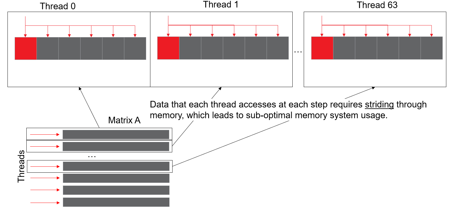
Strided data patterns happen when each thread in a wavefront has to access data locations which have a lot of space between them. For instance, in the algorithm we’ve been using, each thread works on a row, and those rows are contiguous in device memory. This scenario is depicted below:

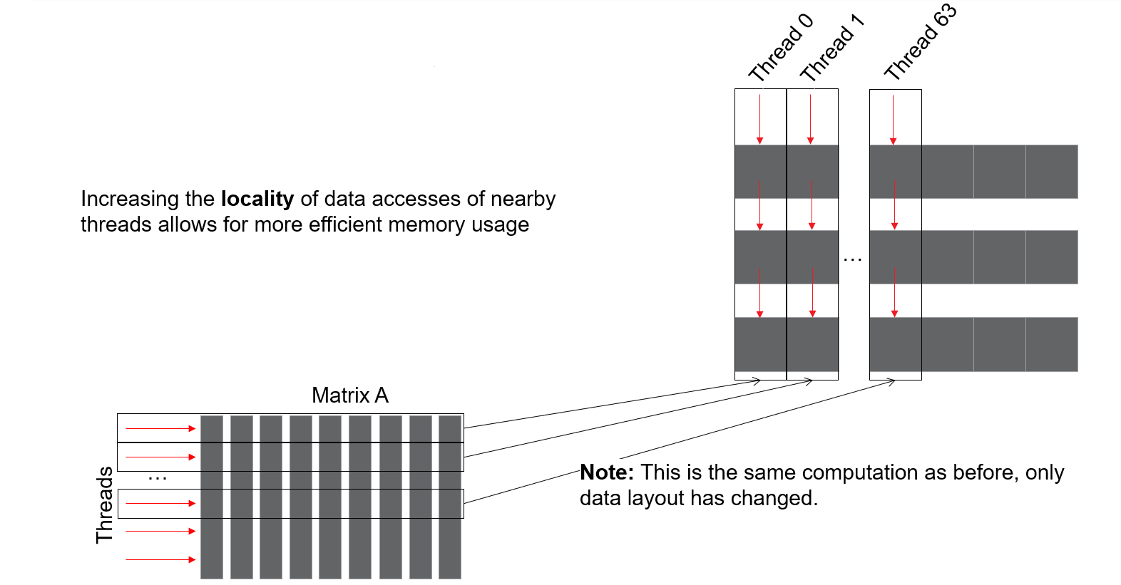
Here the memory addresses accessed by threads at each step of the computation have a lot of space between them, which is suboptimal for memory systems, especially on GPUs. To fix this, we have to re-structure the matrix A so that the columns of the matrix are contiguous, which will result in the rows striding, as seen below:

This new data layout has each block of threads accessing a contiguous chunk of device memory, and will use the memory system of the device much more efficiently. Importantly, the only thing that changed is the physical layout of the memory, so the result of this computation will be the same as the result of the previous data layout.

Initial Roofline Analysis

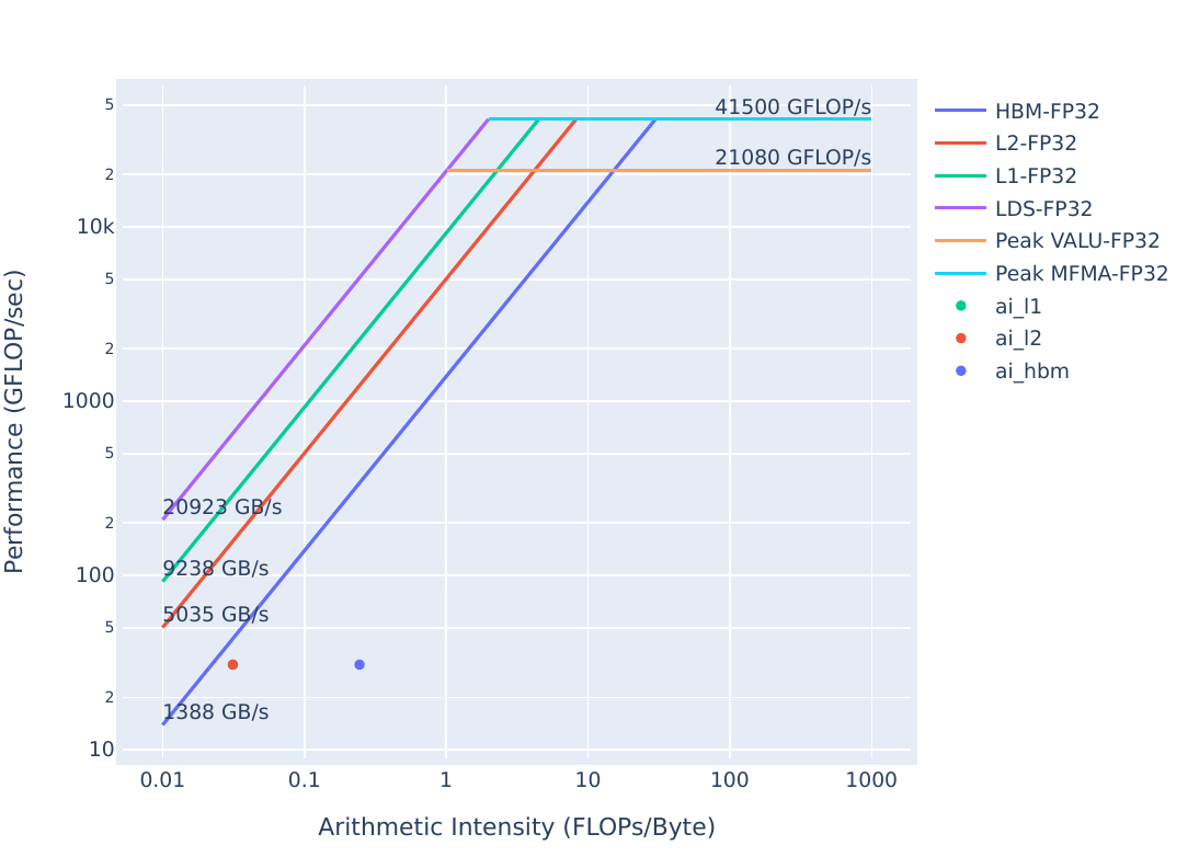
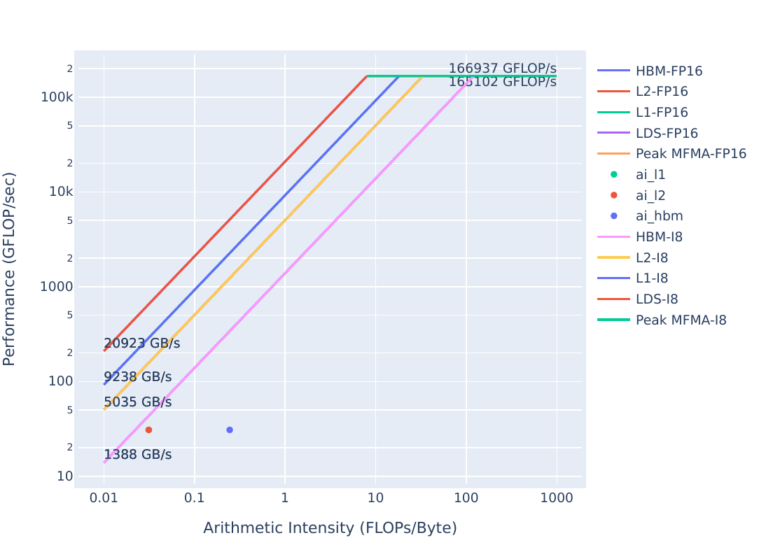
To start, we want to check the roofline of problem.exe, to make sure we are able to improve it. These plots can be generated with:

omniperf profile -n problem_roof_only --roof-only --kernel-names -- ./problem.exe

The plots will appear as PDF files in the ./workloads/problem_roof_only/MI200 directory, if generated on MI200 hardware.

They are also provided below for easy reference:

Roofline Type	Roofline Legend	Roofline Plot
FP32/FP64
FP16/INT8

We have plenty of space to improve this kernel, the next step is profiling.

Exercise Instructions:

To start, let’s build and run the problem executable:

make
./problem.exe

(simulated output)

yAx time: 70 ms

From our other experiments, this time seems reasonable. Let’s look closer at the memory system usage with omniperf:

omniperf profile -n problem --no-roof -- ./problem.exe

(omitted output)

omniperf analyze -p workloads/problem/MI200 --dispatch 1 --block 16.1 17.1

Previous examples have used specific fields inside metrics, but we can also request a group of metrics with just two numbers (i.e. 16.1 vs. 16.1.1)

These requested metrics are: - 16.1 L1 memory speed-of-light stats - 17.1 L2 memory speed-of-light stats

The speed-of-light stats are a more broad overview of how the memory systems are used throughout execution of your kernel. As such, they’re great statistics for seeing if the memory system is generally being used efficiently or not. Output from the analyze command should look like this:

  ___                  _                  __
 / _ \ _ __ ___  _ __ (_)_ __   ___ _ __ / _|
| | | | '_ ` _ \| '_ \| | '_ \ / _ \ '__| |_
| |_| | | | | | | | | | | |_) |  __/ |  |  _|
 \___/|_| |_| |_|_| |_|_| .__/ \___|_|  |_|
                        |_|

Analysis mode = cli
[analysis] deriving Omniperf metrics...

--------------------------------------------------------------------------------
0. Top Stats
0.1 Top Kernels
---------------------------------------------------------------------------------------------------------------
|    | Kernel_Name                              |   Count |     Sum(ns) |    Mean(ns) |   Median(ns) |    Pct |
-----|------------------------------------------|---------|-------------|-------------|--------------|---------
|  0 | yax(double*, double*, double*, int, int, |    1.00 | 70270856.00 | 70270856.00 |  70270856.00 | 100.00 |
|    |  double*) [clone .kd]                    |         |             |             |              |        |
---------------------------------------------------------------------------------------------------------------
0.2 Dispatch List
-------------------------------------------------------------------------------------------------
|    |   Dispatch_ID | Kernel_Name                                                   |   GPU_ID |
-----|---------------|---------------------------------------------------------------|-----------
|  0 |             1 | yax(double*, double*, double*, int, int, double*) [clone .kd] |        8 |
-------------------------------------------------------------------------------------------------


--------------------------------------------------------------------------------
16. Vector L1 Data Cache
16.1 Speed-of-Light
---------------------------------------------------
| Metric_ID   | Metric      |   Avg | Unit        |
--------------|-------------|-------|--------------
| 16.1.0      | Hit rate    |  0.00 | Pct of peak |
--------------|-------------|-------|--------------
| 16.1.1      | Bandwidth   |  8.64 | Pct of peak |
--------------|-------------|-------|--------------
| 16.1.2      | Utilization | 87.71 | Pct of peak |
--------------|-------------|-------|--------------
| 16.1.3      | Coalescing  | 25.00 | Pct of peak |
---------------------------------------------------


--------------------------------------------------------------------------------
17. L2 Cache
17.1 Speed-of-Light
-----------------------------------------------------------------
| Metric_ID   | Metric                        |    Avg | Unit   |
--------------|-------------------------------|--------|---------
| 17.1.0      | Utilization                   |  98.66 | Pct    |
--------------|-------------------------------|--------|---------
| 17.1.1      | Bandwidth                     |  28.10 | Pct    |
--------------|-------------------------------|--------|---------
| 17.1.2      | Hit Rate                      |  93.45 | Pct    |
--------------|-------------------------------|--------|---------
| 17.1.3      | L2-Fabric Read BW             | 125.05 | Gb/s   |
--------------|-------------------------------|--------|---------
| 17.1.4      | L2-Fabric Write and Atomic BW |   0.00 | Gb/s   |
-----------------------------------------------------------------

Looking at this data, we see: - L1 Cache Hit (16.1.0) is 0%, so the kernel’s memory requests are never found in the L1. - L2 Cache Hit (17.1.2) is 93.46%, so most requests are found in the L2, with about 7% needing to go out to HBM. - We are never finding data in the L1 and generating a lot of requests to the L2, so restructuring our data accesses should provide better performance

Since our implementation of yAx simply uses 1 for all values in y, A, and x, we do not have to change how we populate our data. Since A is implemented as a flat array, we don’t need to change our allocation either. >In real-world use-cases, these considerations add non-trivial development overhead, so data access patterns may be non-trivial to change.

To observe the performance effects of a different data access pattern, we simply need to change our indexing scheme. Let’s see how this performs by running solution:

cd solution
make
./solution.exe

(simulated output)

yAx time: 12 ms

We see the runtime here is significantly better than our previous kernel, but we need to check how the caches behave now:

omniperf profile -n solution --no-roof -- ./solution.exe

(output omitted)

omniperf analyze -p workloads/solution/MI200 --dispatch 1 --block 16.1 17.1

The output from this analyze command should look like:

  ___                  _                  __
 / _ \ _ __ ___  _ __ (_)_ __   ___ _ __ / _|
| | | | '_ ` _ \| '_ \| | '_ \ / _ \ '__| |_
| |_| | | | | | | | | | | |_) |  __/ |  |  _|
 \___/|_| |_| |_|_| |_|_| .__/ \___|_|  |_|
                        |_|

Analysis mode = cli
[analysis] deriving Omniperf metrics...

--------------------------------------------------------------------------------
0. Top Stats
0.1 Top Kernels
---------------------------------------------------------------------------------------------------------------
|    | Kernel_Name                              |   Count |     Sum(ns) |    Mean(ns) |   Median(ns) |    Pct |
-----|------------------------------------------|---------|-------------|-------------|--------------|---------
|  0 | yax(double*, double*, double*, int, int, |    1.00 | 12364156.00 | 12364156.00 |  12364156.00 | 100.00 |
|    |  double*) [clone .kd]                    |         |             |             |              |        |
---------------------------------------------------------------------------------------------------------------
0.2 Dispatch List
-------------------------------------------------------------------------------------------------
|    |   Dispatch_ID | Kernel_Name                                                   |   GPU_ID |
-----|---------------|---------------------------------------------------------------|-----------
|  0 |             1 | yax(double*, double*, double*, int, int, double*) [clone .kd] |        8 |
-------------------------------------------------------------------------------------------------


--------------------------------------------------------------------------------
16. Vector L1 Data Cache
16.1 Speed-of-Light
---------------------------------------------------
| Metric_ID   | Metric      |   Avg | Unit        |
--------------|-------------|-------|--------------
| 16.1.0      | Hit rate    | 49.98 | Pct of peak |
--------------|-------------|-------|--------------
| 16.1.1      | Bandwidth   | 12.29 | Pct of peak |
--------------|-------------|-------|--------------
| 16.1.2      | Utilization | 98.12 | Pct of peak |
--------------|-------------|-------|--------------
| 16.1.3      | Coalescing  | 25.00 | Pct of peak |
---------------------------------------------------


--------------------------------------------------------------------------------
17. L2 Cache
17.1 Speed-of-Light
-----------------------------------------------------------------
| Metric_ID   | Metric                        |    Avg | Unit   |
--------------|-------------------------------|--------|---------
| 17.1.0      | Utilization                   |  98.56 | Pct    |
--------------|-------------------------------|--------|---------
| 17.1.1      | Bandwidth                     |  10.03 | Pct    |
--------------|-------------------------------|--------|---------
| 17.1.2      | Hit Rate                      |   0.52 | Pct    |
--------------|-------------------------------|--------|---------
| 17.1.3      | L2-Fabric Read BW             | 694.86 | Gb/s   |
--------------|-------------------------------|--------|---------
| 17.1.4      | L2-Fabric Write and Atomic BW |   0.00 | Gb/s   |
-----------------------------------------------------------------

Looking at this data, we see: - L1 Cache Hit (16.1.0) is around 50%, so half the requests to the L1 need to go to the L2. - L2 Cache Hit (17.1.2) is 0.52%, so almost all the requests to the L2 have to go out to HBM. - L2-Fabric Read BW (17.1.3) has increased significantly, due to the increase in L2 cache misses requiring HBM reads.

Solution Roofline Analysis

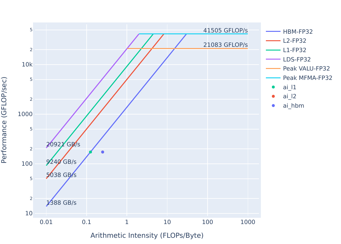
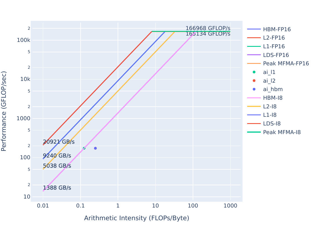
We should check where our new kernel stands on the roofline. These plots can be generated with:

omniperf profile -n solution_roof_only --roof-only --kernel-names -- ./solution.exe

The plots will appear as PDF files in the ./workloads/problem_roof_only/MI200 directory, if generated on MI200 hardware.

They are also provided below for easy reference:

Roofline Type	Roofline Legend	Roofline Plot
FP32/FP64
FP16/INT8

We appear to be very close to being bound by the HBM bandwidth from the fp32 roofline. To get more performance we need to look closer at our algorithm.

Roofline Comparison

Roofline Type	Problem Roofline	Solution Roofline
FP32/FP6
FP16/INT8

We see that the HBM roofline point moves up, while the L1/L2 points move up and to the right from problem to solution. This means that our arithmetic intensity is increasing for the caches, so we are moving less data through the caches to do the same computation.

Summary and Take-aways

This exercise illustrates the at times insidious nature of strided data access patterns. They can be difficult to spot in code, but profiling more readily shows when adversarial access patterns occur, by showing poor cache hit rates, low cache bandwidth, and potentially low utilization. Data access patterns can be non-trivial to change, so these sorts of optimizations can involve significant development and validation overhead.