
Generate SSH key as shown below
cd $HOME
ssh-keygen -t ed25519 -N ''
cat $HOME/.ssh/id_ed25519.pubssh <username>@aac1.amd.com -i id_ed25519 -p #### The port number will be established when the container environment starts up and will be given out at that time.
At first login, you will be presented with the AMD Accelerator Cloud (AAC) use agreement form. It covers the terms of use of the compute hardware as well as how we will handle your data.
To simplify the login even further, you can add the following to your .ssh/config file.
The ServerAlive* lines in the config file may be added to avoid timeouts when idle.
# AMD AAC cluster
Host aac
   User <USERNAME>
   Hostname aac1.amd.com
   IdentityFile id_ed25519 -- can put full path as well -- $HOME/.ssh/id_ed25519
   Port #### -- but this might change, so add on the command line shown below
   ServerAliveInterval 600
   ServerAliveCountMax 30
and then login using
ssh aac -p ####If when executing the above command, you get an error saying that the key file does not exist, you may have to write explicitly into the .ssh/config file what $HOME is. It may also happen that a message like the following will show after logging into AAC:
@@@@@@@@@@@@@@@@@@@@@@@@@@@@@@@@@@@@@@@@@@@@@@@@@@@@@@@@@@@
@    WARNING: REMOTE HOST IDENTIFICATION HAS CHANGED!     @
@@@@@@@@@@@@@@@@@@@@@@@@@@@@@@@@@@@@@@@@@@@@@@@@@@@@@@@@@@@
IT IS POSSIBLE THAT SOMEONE IS DOING SOMETHING NASTY!
Someone could be eavesdropping on you right now (man-in-the-middle attack)!
It is also possible that a host key has just been changed.
In this case, it may be necessary to remove in your local system the offending keys located in .ssh/known_hosts, as indicated by the warning message.
Persistent storage is at /datasets/teams/hackathon-testing/<userid>. Your home directory will be set to this directory.
$HOME=/datasets/teams/hackathon-testing/<userid>Files in that directory will persist across container starts and stops and even be available from another container with the same userid on systems at the same hosting location.
You can copy files in or out with the scp or the rsync command.
Copy into AAC from your local system
scp -i <path>/<keyfile> -P #### <file> USER@aac1.amd.com:~/<path>/<file>Copy from AAC to your local system
scp -i <path>/<keyfile> -P #### USER@aac1.amd.com:~/path/to/your/file ./To copy files in or out of the container, you can also use rsync as shown below:
rsync -avz -e "ssh -i <path>/<keyfile> -p ####" <file> <USER>@aac1.amd.com:~/path/to/your/filesThis container is based on the Ubuntu 22.04 Operating System with the ROCm 5.7.2 software stack. It contains multiple versions of AMD, GCC, and LLVM compilers, hip libraries, GPU-Aware MPI (OpenMPI and MVAPICH), and AMD Profiling tools with perfetto and graphana. The container also has modules set up with the lua modules package and a slurm package and configuration. It includes the following additional packages:
module avail Output list of modules avail command
----------------------------- /etc/lmod/modules/Linux ------------------------------------------
clang/base    clang/14    clang/15 (D)    gcc/base    gcc/11 (D)    gcc/12    gcc/13    miniconda/23.11.0
----------------------------- /etc/lmod/modules/ROCm -------------------------------------------
amdclang/17.0-6.0.2    hipfort/6.0.2    opencl/6.0.2    rocm/6.0.2
----------------------------- /etc/lmod/modules/ROCmPlus-MPI -----------------------------------
mvapich2/2.3.7    openmpi/5.0.0
----------------------------- /etc/lmod/modules/ROCmPlus-AMDResearchTools ----------------------
omniperf/2.0.0    omnitrace/1.11.1
----------------------------- /etc/lmod/modules/ROCmPlus-LatestCompilers -----------------------
  amd-gcc/13.2.0    aomp/amdclang-18.0    clacc/clang-17.0.0    llvm-latest/gcc11_hipstdpar    og/gcc-develop-24-02-27
----------------------------- /etc/lmod/modules/ROCmPlus-AI -----------------------
cupy/13.0.0b1    pytorch/2.2
----------------------------- /usr/share/lmod/lmod/modulefiles ---------------------------------
Core/lmod/6.6    Core/settarg/6.6
Where:   D:  Default Module
There are three modules associated with each ROCm version. One is the rocm module which is needed by many of the other modules. The second is the amdclang module when using the amdclang compiler that comes bundled with ROCm. The third is the hipfort module for the Fortran interfaces to HIP.
Compiler modules set the C, CXX, FC flags. Only one compiler module can be loaded at a time. hipcc is in the path when the rocm module is loaded. Note that there are several
The SLURM configuration is for a single queue that is shared with the rest of the node.
sinfo | PARTITION | AVAIL | TIMELIMIT | NODES | STATE | NODELIST |
|---|---|---|---|---|---|
| LocalQ | up | 2:00:00 | 1 | idle | localhost |
The SLURM salloc command may be used to acquire a long term session that exclusively grants access to one or more GPUs. Alternatively, the srun or sbatch commands may be used to acquire a session with one or more GPUs and only exclusively use the session for the life of the run of an application. squeue and sinfo will show information about the current state of the SLURM system.
The exercise examples are preloaded into the /Shared directory. Copy the files into your home directory with
mkdir -p $HOME/HPCTrainingExamples
scp -pr /Shared/HPCTrainingExamples/* $HOME/HPCTrainingExamples/
If you need to refer to the examples separately, they are at the repository below.
Alternatively, you can get the examples from our repo. This repo contains all the code that we will use for the exercises that follow
cd $HOME
git clone https://github.com/amd/HPCTrainingExamples.gitThe source code for these exercises is based on those in the presentation, but with details filled in so that there is a working code. You may want to examine the code in these exercises and compare it to the code in the presentation and to the code in the other exercises.
git clone https://github.com/amd/HPCTrainingExamples.git
cd HPCTrainingExamples/ManagedMemory
First run the standard CPU code. This is a working version of the original CPU code from the programming model presentation.
cd HPCTrainingExamples/ManagedMemory/CPU_Code
module load amdclang
make
will compile with amdclang -g -O3 -fopenmp cpu_code.c -o cpu_code Then run code with
./cpu_codeThis example adds the GPU memory corresponding to the CPU arrays and explicitly manages the memory transfers.
cd ../GPU_Code
make
This will compile with hipcc -g -O3 -fopenmp --offload-arch=gfx90a gpu_code.hip -o gpu_code Then run the code with
./gpu_codeIn this example, we will set the HSA_XNACK environment variable to 1 and let the Operating System move the memory for us.
export HSA_XNACK=1
cd ../Managed_Memory_Code
make
./gpu_codeThis example is shown on slide 29. We’ll run the same code as we used in the managed memory example. Because the memory pointers are addressable on both the CPU and the GPU, no memory managment is necessary. First, log onto an MI300A node. Then compile and run the code as follows.
cd ../APU_Code
make
./gpu_codeFor this example, we have a simple code with the loop offloading in the main code, openmp_code, and a second version, openmp_code1, with the offloaded loop in a subroutine where the compiler cannot tell the size of the array. Running this on the MI200 series, it passes, despite that it does not have a single address space. We add export LIBOMPTARGET_INFO=-1 to verify that it is running on the GPU.
export HSA_XNACK=1
module load amdclang
cd ../OpenMP_Code
make
./openmp_code
./openmp_code1
export LIBOMPTARGET_INFO=-1
./openmp_code
./openmp_code1
For more experimentation with this example, comment out the first line of the two source codes.
//#pragma omp requires unified_shared_memory
make
export LIBOMPTARGET_INFO=-1
./openmp_code
./openmp_code1
Now with the LIBOMPTARGET_INFO variable set, we get a report that memory is being copied to the device and back. The OpenMP compiler is helping out a lot more than might be expected even without an APU.
First, set up the environment
module load amdclang
module load rocm
For the Raja example, we need to build the Raja code first
cd ~/HPCTrainingExamples/ManagedMemory/Raja_Code

PWDir=`pwd`

git clone --recursive https://github.com/LLNL/RAJA.git Raja_build
cd Raja_build

mkdir build_hip && cd build_hip

cmake -DCMAKE_INSTALL_PREFIX=${PWDir}/Raja_HIP \
      -DROCM_ROOT_DIR=/opt/rocm \
      -DHIP_ROOT_DIR=/opt/rocm \
      -DHIP_PATH=/opt/rocm/bin \
      -DENABLE_TESTS=Off \
      -DENABLE_EXAMPLES=Off \
      -DRAJA_ENABLE_EXERCISES=Off \
      -DENABLE_HIP=On \
      ..

make -j 8
make install

cd ../..

rm -rf Raja_build

export Raja_DIR=${PWDir}/Raja_HIP
Now we build the example. Note that we just allocated the arrays on the host with malloc. To run it on the MI200 series, we need to set the HSA_XNACK variable.
# To run with managed memory
export HSA_XNACK=1

mkdir build && cd build
CXX=hipcc cmake ..
make
./raja_code

cd ..
rm -rf build

cd ${PWDir}
rm -rf Raja_HIP

cd ..
rm -rf ${PROB_NAME}First, set up the environment
module load amdclang
module load rocm
For the Kokkos example, we need to build the Kokkos code first
cd ~/HPCTrainingExamples/ManagedMemory/Kokkos_Code

PWDir=`pwd`

git clone https://github.com/kokkos/kokkos Kokkos_build
cd Kokkos_build

mkdir build_hip && cd build_hip
cmake -DCMAKE_INSTALL_PREFIX=${PWDir}/Kokkos_HIP -DKokkos_ENABLE_SERIAL=ON \
      -DKokkos_ENABLE_HIP=ON -DKokkos_ARCH_ZEN=ON -DKokkos_ARCH_VEGA90A=ON \
      -DCMAKE_CXX_COMPILER=hipcc ..

make -j 8
make install

cd ../..

rm -rf Kokkos_build

export Kokkos_DIR=${PWDir}/Kokkos_HIP
Now we build the example. Note that we have not had to declare the arrays in Kokkos Views. To run it on the MI200 series, we need to set the HSA_XNACK variable.
# To run with managed memory
export HSA_XNACK=1

mkdir build && cd build
CXX=hipcc cmake ..
make
./kokkos_code

cd ${PWDir}
rm -rf Kokkos_HIP

cd ..
rm -rf ${PROB_NAME} %------------------------%Running the first OpenMP example: Pragma_Examples/OpenMP/C/Make/saxpy
module load amdclang
make clean
make
./saxpy
Confirm running on GPU with
export LIBOMPTARGET_KERNEL_TRACE=1
./saxpyAMD_LOG_LEVEL=[0|1|2|3|4] or LIBOMPTARGET_KERNEL_TRACE=2We start out with the OpenMP threaded code for the CPU. This code is in ~/HPCTrainingExamples/Pragma_Examples/OpenMP/Intro in the saxpy_cpu.cpp file. This is the code on slide 16. We first load the amdclang module which will set the CXX environment variable. This variable will get picked up by the Makefile for the build.
module load amdclang
make saxpy_cpu
./saxpy_cpu
The next example, saxpy1, is from slide 18 where the first version of OpenMP offloading is tried. In this code, there is no map clause. The compiler can figure out the arrays that need to be copied over and their sizes.
make saxpy1
./saxpy1
While running one of these codelets, it may be useful to watch the GPU usage. Here are two approaches.
open another terminal and ssh to the AAC node you are working on, or
use the tmux command
run watch -n 0.5 rocm-smi command line from that terminal to visualize GPU activities.
Note that the basic tmux survival commands are:
cntl+b \"  - splits the screen
cntl+b (up arrow) - move to the upper session
cntl+b (down arrow) - move to lower session
exit - end tmux session
Next, run the codelet on your preferred GPU device if you have allocated more than 1 GPU. For example, to execute on GPU ID #2, set the following environment variable: export ROCR_VISIBLE_DEVICES=2 then run the code.
Profile the codelet and then compare output by setting
export LIBOMPTARGET_KERNEL_TRACE=1
export LIBOMPTARGET_KERNEL_TRACE=2
Note:
rocminfo can be used to get target architecture information.
The Fortran version of the saxpy code is shown in saxpy1f.F90. It is very similar to the C and C++ OpenMP pragmas. In Fortran, the compiler hints are technically directives that are contained in specially formatted comments. One of the strengths of OpenMP is that the language can be used in C, C++, and Fortran code and they can even be mixed in an application. Here is how to run the Fortran example.
make saxpy1f
./saxpy1f
The compile line uses the specific GPU architecture type. It grabs it from the rocminfo command with a little bit of string manipulation.
Let’s now add a map clause as shown in quotes on slide 18 – map(tofrom:y[0:N])
make saxpy2
./saxpy2
A lot of the initial optimization of an OpenMP offloading port is to minimize the data movement from host to device and back. What is the optimum mapping of data for this example? See saxpy3.cpp for the optimal map clauses.
make saxpy3
./saxpy3
In the example we have been working with so far, the compiler can determine the sizes and will move the data for you. Let’s see what happens when we have a subroutine with pointers where the compiler does not know the sizes.
make saxpy4
./saxpy4
Try removing the map clause – the program will now fail.
We have been running on the GPU, but with only one thread in serial. Let’s start adding parallelism. The first thing we can do is add #pragma omp parallel for simd before the loop to tell it to run in parallel.
make saxpy5
./saxpy5
We have told it to run the loop in parallel, but we haven’t given it any hardware resources. To add more compute units, we need to add the teams clause. Then to spread the work across the threads, we need the distribute clause. (This code is currently not working …)
make saxpy6
./saxpy6
More commonly, we add the triplet of target teams distribute to the pragma to enable all hardware elements to the computation.
make saxpy7
./saxpy7
And in Fortran.
make saxpy2f
./saxpy2fThis example from slide 29 shows the use of a structured block region that encompasses several compute loops. The data region persists across all of them, eliminating the need for map clauses and data transfers.
make target_data_structured
./target_data_structured
This example shows the use of the target data to map the data to the device and then updating it with the target update in the middle of the target data block.
make target_data_unstructured
./target_data_unstructured
When using larger data regions, it can be necessary to move data in the middle of the region to support MPI communication or I/O. This example shows the use of the update clause to copy new input from the host to the device.
make target_data_update
./target_data_update %------------------------%The first example is a simple reduction, similar to what we have done before
module load amdclang
git clone https://github.com/AMD/HPCTrainingExamples
cd ~/HPCTrainingExamples/Pragma_Examples/OpenMP/Fortran
cd reduction_scalar
make
./reduction_scalar
Now try the array form
cd ../reduction_array
make
./reduction_array
If your compiler passes, it supports at least simple array reduction clauses
Subroutines called from within a target region also cause some difficulties. We must tell the compiler that we want these compiled for the GPU. For this example
cd ../device_routine
make
./device_routineIncluding the use of data from global scope in device routines also causes difficulties. We have examples for both statically sized arrays and dynamically allocated global data.
cd ../device_routine_wglobaldata
make
./device_routine
cd ../device_routine_wdynglobaldata
make
./device_routineIt is suggested for those that want to truly experience the effort, that you take all the pragma statements out of these examples and do the port yourself
%------------------------%Setup your environment
export LIBOMPTARGET_INFO=-1
export OMP_TARGET_OFFLOAD=MANDATORY
You can also be more selective in the output generated by using the individual bit masks
export LIBOMPTARGET_INFO=$((0x01 | 0x02 | 0x04 | 0x08 | 0x10 | 0x20))The first example code uses just a single pragma with a map clause at the computational loop. Examine this code and then compile and run.
mkdir build && cd build
cmake ..
make
./mem1
You should get some output like the following
Libomptarget device 0 info: Entering OpenMP kernel at mem1.cc:89:1 with 5 arguments:
Libomptarget device 0 info: firstprivate(n)[4] (implicit)
Libomptarget device 0 info: from(z[0:n])[80000]
Libomptarget device 0 info: firstprivate(a)[8] (implicit)
Libomptarget device 0 info: to(x[0:n])[80000]
Libomptarget device 0 info: to(y[0:n])[80000]
Libomptarget device 0 info: Creating new map entry with HstPtrBase=0x0000000001772200, ...
Libomptarget device 0 info: Creating new map entry with HstPtrBase=0x000000000174b0e0, ...
Libomptarget device 0 info: Copying data from host to device, HstPtr=0x000000000174b0e0, ...
Libomptarget device 0 info: Creating new map entry with HstPtrBase=0x000000000175e970, ...
Libomptarget device 0 info: Copying data from host to device, HstPtr=0x000000000175e970, ...
Libomptarget device 0 info: Mapping exists with HstPtrBegin=0x0000000001772200, ...
Libomptarget device 0 info: Mapping exists with HstPtrBegin=0x000000000174b0e0, ...
Libomptarget device 0 info: Mapping exists with HstPtrBegin=0x000000000175e970, ...
Libomptarget device 0 info: Mapping exists with HstPtrBegin=0x000000000175e970, ...
Libomptarget device 0 info: Mapping exists with HstPtrBegin=0x000000000174b0e0, ...
Libomptarget device 0 info: Mapping exists with HstPtrBegin=0x0000000001772200, ...
Libomptarget device 0 info: Copying data from device to host, TgtPtr=0x00007f617c420000, ...
Libomptarget device 0 info: Removing map entry with HstPtrBegin=0x000000000175e970, ...
Libomptarget device 0 info: Removing map entry with HstPtrBegin=0x000000000174b0e0, ...
Libomptarget device 0 info: Removing map entry with HstPtrBegin=0x0000000001772200, ...
-Timing in Seconds: min=0.010115, max=0.010115, avg=0.010115
-Overall time is 0.010505
Last Value: z[9999]=7.000000
Explore examples 2 through 5 and observe the output produced when the LIBOMPTARGET_INFO environment variable is set.
Mem2 pattern : Add enter/exit data alloc/delete when memory is created/freed
After new
mem2.cc:#pragma omp target enter data map(alloc: x[0:n], y[0:n], z[0:n])
Loop around computational loop and keep map on computational loop. The map to/from should check if the data exists. If not, it will allocate/delete it. Then it will do the copies to and from. This will increment the Reference Counter and decrement it at end of loop.
mem2.cc:#pragma omp target teams distribute parallel for simd map(to: x[0:n], y[0:n]) map(from: z[0:n])
Before delete
mem2.cc:#pragma omp target exit data map(delete: x[0:n], y[0:n], z[0:n])
Mem3 pattern: Replacing map to/from with updates to bypass unneeded device memory check
After new
mem3.cc:#pragma omp target enter data map(alloc: x[0:n], y[0:n], z[0:n])
Before computational loop. Data should be copied. Reference counter should not change.
   mem3.cc:#pragma omp target update to (x[0:n], y[0:n])
   mem3.cc:#pragma omp target teams distribute parallel for simd
After computational loop
mem3.cc:#pragma omp target update from (z[0:n])
Before delete
mem3.cc:#pragma omp target exit data map(delete: x[0:n], y[0:n], z[0:n])
Mem4 pattern: Replacing delete with release to use Reference Counting
   mem4.cc:#pragma omp target enter data map(alloc: x[0:n], y[0:n], z[0:n])
   mem4.cc:#pragma omp target exit data map(release: x[0:n], y[0:n], z[0:n])
   mem4.cc:#pragma omp target teams distribute parallel for simd map(to: x[0:n], y[0:n]) map(from: z[0:n])
Mem5 pattern: Using enter data map to/from alloc/delete to reduce memory copies
   mem5.cc:#pragma omp target enter data map(to: x[0:n], y[0:n]) map(alloc: z[0:n])
   mem5.cc:#pragma omp target exit data map(from: z[0:n]) map(delete: x[0:n], y[0:n])
mem5.cc:#pragma omp target teams distribute parallel for simd map(to:x[0:n], y[0:n]) map(from: z[0:n])Mem6 pattern: Using enter data alloc/delete with update clause at end
   mem6.cc:#pragma omp target enter data map(alloc: x[0:n], y[0:n], z[0:n])
   mem6.cc:#pragma omp target teams distribute parallel for simd
   mem6.cc:#pragma omp target update from(z[0])
   mem6.cc:#pragma omp target exit data map(delete: x[0:n], y[0:n], z[0:n])
mem6.cc:#pragma omp target teams distribute parallel for simdMem7 pattern: Using Unified Shared Memory to automatically move data
   mem7.cc:#pragma omp requires unified_shared_memory
   mem7.cc:#pragma omp target teams distribute parallel for simd
   mem7.cc:#pragma omp target teams distribute parallel for simd
For this example, HSA_XNACK=1 needs to be set
export HSA_XNACK=1
make mem7
./mem7Mem8 pattern: Demonstrating Unified Shared Memory with maps for backward compatibility
   set HSA_XNACK=1 at runtime

   mem8.cc:#pragma omp requires unified_shared_memory
   mem8.cc:#pragma omp target enter data map(alloc: x[0:n], y[0:n], z[0:n])
   mem8.cc:#pragma omp target teams distribute parallel for simd
   mem8.cc:#pragma omp target update from(z[0])
   mem8.cc:#pragma omp target exit data map(delete: x[0:n], y[0:n], z[0:n])
mem8.cc:#pragma omp target teams distribute parallel for simdWe now switch to how unified address programming would look in other languages. The language we will work with the most will be OpenMP. We’ll start by looking at the unified address code shown in slide 31 and 32. It is also in the mem12.cc file in the directory given below. You should also compare it to the original GPU code using explicit memory management in mem1.cc through mem6.cc.
We’ll now run the unified address example if we have access to an MI300A GPU. If you don’t have access to an MI300A, we’ll also run nearly the same code in mem7.cc with managed memory on the MI200 series GPUs. We’ll be looking at all of the versions of this code in the Advanced OpenMP presentation.
cd ~/HPCTrainingExamples/Pragma_Examples/OpenMP/CXX/memory_pragmas
module load amdclang
make mem12
./mem12Download the exercises and go to the directory with the kernel pragma examples
git clone https://github.com/amd/HPCTrainingExamples.git
cd HPCTrainingExamples/Pragma_Examples/OpenMP/CXX/kernel_pragmas
Setup your environment. You should unset the LIBOMPTARGET_INFO environment from previous exercise.
unset LIBOMPTARGET_INFOexport CXX=amdclang++
export LIBOMPTARGET_KERNEL_TRACE=1
export OMP_TARGET_OFFLOAD=MANDATORY
export HSA_XNACK=1The base version 1 code is the Unified Shared memory example from the previous exercises
mkdir build && cd build
cmake ..
make kernel1
./kernel1
Kernel2 : add num_threads(64)
Kernel3 : add num_threads(64) thread_limit(64)
On your own: Uncomment line in CMakeLists.txt with -faligned-allocation -fnew-alignment=256
Another option is to add the attribute (std::align_val_t(128) ) to each new line. For example:
double *x = new (std::align_val_t(128) ) double[n];git clone https://github.com/amd/HPCTrainingExamples.git
For the first interactive example, get an slurm interactive session
salloc -N 1 -p LocalQ --gpus=1 -t 10:00
cd HPCTrainingExamples/HIP/vectorAdd
Examine files here - README, Makefile, CMakeLists.txt and vectoradd.hip. Notice that Makefile requires ROCM_PATH to be set. Check with module show rocm or echo $ROCM_PATH Also, the Makefile builds and runs the code. We’ll do the steps separately. Check also the HIPFLAGS in the Makefile. There is also a CMakeLists.txt file to use for a cmake build.
For the portable Makefile system
module load rocm

make vectoradd
./vectoradd
Pro tip for Makefile builds. Run make clean before make to be sure nothing is left over from a previous build.
This example also runs with the cmake system
module load rocm

mkdir build && cd build
cmake ..
make
./vectoradd
Pro tip for cmake builds. To rebuild after changing CMake options or using a different compiler, either
We can use a SLURM submission script, let’s call it hip_batch.sh. There is a sample script for some systems in the example directory.
#!/bin/bash
#SBATCH -N 1
#SBATCH -p LocalQ
#SBATCH --gpus=1
#SBATCH -t 10:00

module load rocm
cd $HOME/HPCTrainingExamples/HIP/vectorAdd

make vectoradd
./vectoradd
Submit the script sbatch hip_batch.sh
Check for output in slurm-<job-id>.out or error in slurm-<job-id>.err
To use the cmake option in the batch file, change the build to
mkdir build && cd build
cmake ..
make
./vectoradd
Now let’s try the hip-stream example. This example is from the original McCalpin code as ported to CUDA by Nvidia. This version has been ported to use HIP.
module load rocm
cd $HOME/HPCTrainingExamples/HIP/hip-stream
make
./stream
Note that it builds with the hipcc compiler. You should get a report of the Copy, Scale, Add, and Triad cases.
On your own:
HPCTrainingExamples/HIPHIPCC=nvcc before the make command or -DCMAKE_GPU_RUNTIME=CUDA to the cmake command. (See README file)The jacobi example has a more complex build that incorporates MPI. The original Makefile has not been modified, but a CMakeLists.txt has been added to demonstrate a portable cmake build. From an interactive session, build the example.
cd $HOME/HPCTrainingExamples/HIP/jacobi

module load rocm
module load openmpi

mkdir build && cd build
cmake ..
make
Since we will be running on two MPI ranks, you will need to alloc 2 GPUs for a quick run. Exit your current allocation with exit and then get the two GPUs. Keep the requested time short to avoid tying up the GPUs so others can run the examples. The requested time shown is in the format hours:minutes:seconds so it is for one minute.
salloc -p LocalQ --gpus=2 -n 2 -t 00:01:00
module load rocm openmpi
mpirun -n 2 ./Jacobi_hip -g 2Choose one or more of the CUDA samples in HPCTrainingExamples/HIPIFY/mini-nbody/cuda directory. Manually convert it to HIP. Tip: for example, the cudaMalloc will be called hipMalloc. You can choose from nbody-block.cu, nbody-orig.cu, nbody-soa.cu
You’ll want to compile on the node you’ve been allocated so that hipcc will choose the correct GPU architecture.
Use the hipify-perl script to “hipify” the CUDA samples you used to manually convert to HIP in Exercise 1. hipify-perl is in $ROCM_PATH/hip/bin directory and should be in your path.
First test the conversion to see what will be converted
hipify-perl -examine nbody-orig.cuYou’ll see the statistics of HIP APIs that will be generated. The output might be different depending on the ROCm version.
[HIPIFY] info: file 'nbody-orig.cu' statistics:
  CONVERTED refs count: 7
  TOTAL lines of code: 91
  WARNINGS: 0
[HIPIFY] info: CONVERTED refs by names:
  cudaFree => hipFree: 1
  cudaMalloc => hipMalloc: 1
  cudaMemcpyDeviceToHost => hipMemcpyDeviceToHost: 1
  cudaMemcpyHostToDevice => hipMemcpyHostToDevice: 1
hipify-perl is in $ROCM_PATH/hip/bin directory and should be in your path. In some versions of ROCm, the script is called hipify-perl.
Now let’s actually do the conversion.
hipify-perl nbody-orig.cu > nbody-orig.cppCompile the HIP programs.
hipcc -DSHMOO -I ../ nbody-orig.cpp -o nbody-origThe #define SHMOO fixes some timer printouts. Add --offload-arch=<gpu_type> to specify the GPU type and avoid the autodetection issues when running on a single GPU on a node.
Run the program
./nbody-origA batch version of Exercise 2 is:
#!/bin/bash
#SBATCH -N 1
#SBATCH --ntasks=1
#SBATCH --gpus=1
#SBATCH -p LocalQ
#SBATCH -t 00:10:00

pwd
module load rocm

cd HPCTrainingExamples/HIPIFY/mini-nbody/cuda
hipify-perl -print-stats nbody-orig.cu > nbody-orig.cpp
hipcc -DSHMOO -I ../ nbody-orig.cpp -o nbody-orig
./nbody-orig
Notes:
hipconvertinplace-perl is a convenience script that does hipify-perl -inplace -print-stats commandLoad the proper environment
cd $HOME/HPCTrainingExamples/HIPFY/
module load rocm
Get the CUDA version of the Pennant mini-app.
wget https://asc.llnl.gov/sites/asc/files/2020-09/pennant-singlenode-cude.tgz
tar -xzvf pennant-singlenode-cude.tgz

cd PENNANT

hipexamine-perl.sh
And review the output
Now do the actual conversion. We want to do the conversion for the whole directory tree, so we’ll use hipconvertinplace-sh
hipconvertinplace-perl.shWe want to use .hip extensions rather than .cu, so change all files with .cu to .hip
mv src/HydroGPU.cu src/HydroGPU.hipNow we have two options to convert the build system to work with both ROCm and CUDA
First cut at converting the Makefile. Testing with make can help identify the next step.
clang++ located in ${ROCM_PATH}/llvm/bin/clang++-fast and -fno-alias from the CXXFLAGS_OPT.cu to .hip in the MakefileNow we are just getting compile errors from the source files. We will have to do fixes there. We’ll tackle them one-by-one.
The first errors are related to the double2 type.
compiling src/HydroGPU.hip
(CPATH=;hipcc -O3 -I.  -c -o build/HydroGPU.o src/HydroGPU.hip)
In file included from src/HydroGPU.hip:14:
In file included from src/HydroGPU.hh:16:
src/Vec2.hh:35:8: error: definition of type 'double2' conflicts with type alias of the same name
struct double2
       ^
/opt/rocm-5.6.0/include/hip/amd_detail/amd_hip_vector_types.h:1098:1: note: 'double2' declared here
__MAKE_VECTOR_TYPE__(double, double);

^
/opt/rocm-5.6.0/include/hip/amd_detail/amd_hip_vector_types.h:1062:15: note: expanded from macro '__MAKE_VECTOR_TYPE__'
        using CUDA_name##2 = HIP_vector_type<T, 2>;\

              ^
<scratch space>:316:1: note: expanded from here
double2
HIP defines double2. Let’s look at Vec2.hh. At line 33 where the first error occurs. We see an #ifdef __CUDACC__ around a block of code there. We also need the #ifdef to include HIP as well. Let’s check the available compiler defines from the presentation to see what is available. It looks like we can use __HIP_DEVICE_COMPILE__ or maybe __HIPCC__.
Change line 33 in Vec2.hh to #ifndef __HIPCC__
The next error is about function attributes that are incorrect for device code.
compiling src/HydroGPU.hip
(CPATH=;hipcc -O3 -I.  -c -o build/HydroGPU.o src/HydroGPU.hip
src/HydroGPU.hip:168:23: error: no matching function for call to 'cross
    double sa = 0.5 * cross(px[p2] - px[p1],  zx[z] - px[p1]);
                      ^~~~
src/Vec2.hh:206:15: note: candidate function not viable: call to __host__ function from __device__ function
The FNQUALIFIER macro is what handles the attributes in the code. We find that defined at line 22 and again we see a #ifdef __CUDACC__. It is another #ifdef __CUDACC__. We can see that we need to pay attention to all the CUDA ifdef statements.
Change line 22 to #ifdef __HIPCC__
Finally we get an error about already defined operators on double2 types. These appear to be defined in HIP, but not in CUDA. So we change line 84
compiling src/HydroGPU.hip
(CPATH=;hipcc -O3 -I.  -c -o build/HydroGPU.o src/HydroGPU.hip)
src/HydroGPU.hip:149:15: error: use of overloaded operator '+=' is ambiguous (with operand types 'double2' (aka 'HIP_vector_type<double, 2>') and 'double2')
        zxtot += ctemp2[sn];
        ~~~~~ ^  ~~~~~~~~~~
/opt/rocm-5.6.0/include/hip/amd_detail/amd_hip_vector_types.h:510:26: note: candidate function
        HIP_vector_type& operator+=(const HIP_vector_type& x) noexcept
                         ^
src/Vec2.hh:88:17: note: candidate function
inline double2& operator+=(double2& v, const double2& v2)
Change line 85 to #elif defined(__CUDACC__)
Now we start getting errors for HydroGPU.hip. The first is for the atomicMin function. It is already defined in HIP, so we need to add an ifdef for CUDA around the code.
compiling src/HydroGPU.hip
(CPATH=;hipcc -O3 -I.  -c -o build/HydroGPU.o src/HydroGPU.hip)
src/HydroGPU.hip:725:26: error: static declaration of 'atomicMin' follows non-static declaration
static __device__ double atomicMin(double* address, double val)
                         ^
/opt/rocm-5.6.0/include/hip/amd_detail/amd_hip_atomic.h:478:8: note: previous definition is here
double atomicMin(double* addr, double val) {                                                                                                                          ^
       ^
1 error generated when compiling for gfx90a.
Add #ifdef __CUDACC__/endif to the more block of code in HydroGPU.hip from line 725 to 737
We finally got through the compiler errors and move on to link errors
linking build/pennant/opt/rocm-5.6.0//llvm/bin/clang++ -o build/pennant build/ExportGold.o build/ImportGMV.o build/Parallel.o build/WriteXY.o build/HydroBC.o build/QCS.o build/TTS.o build/main.o build/Mesh.o build/InputFile.o build/GenMesh.o build/Driver.o build/Hydro.o build/PolyGas.o build/HydroGPU.o -L/lib64 -lcudart
ld.lld: error: unable to find library -lcudartIn the Makefile, change the LDFLAGS while keeping the old settings for when we set up the switch between GPU platforms.
LDFLAGS_CUDA := -L$(HIP_INSTALL_PATH)/lib64 -lcudart
LDFLAGS := -L${ROCM_PATH}/hip/lib -lamdhip64
We then get the link error
linking build/pennant/opt/rocm-5.6.0//llvm/bin/clang++ -o build/pennant build/ExportGold.o build/ImportGMV.o build/Parallel.o build/WriteXY.o build/HydroBC.o build/QCS.o build/TTS.o build/main.o build/Mesh.o build/InputFile.o build/GenMesh.o build/Driver.o build/Hydro.o build/PolyGas.o build/HydroGPU.o -L/opt/rocm-5.6.0//hip/lib -lamdhip64
ld.lld: error: undefined symbol: hydroInit(int, int, int, int, int, double, double, double, double, double, double, double, double, double, int, double const*, int, double const*, double2 const*, double2 const*, double const*, double const*, double const*, double const*, double const*, double const*, double const*, int const*, int const*, int const*, int const*, int const*, int const*)
>>> referenced by Hydro.cc
>>>               build/Hydro.o:(Hydro::Hydro(InputFile const*, Mesh*))

ld.lld: error: undefined symbol: hydroGetData(int, int, double2*, double*, double*, double*)
>>> referenced by Hydro.cc
>>>               build/Hydro.o:(Hydro::getData())
This one is a little harder. We can get more information by using nm build/Hydro.o |grep hydroGetData and nm build/HydroGPU.o |grep hydroGetData. We can see that the subroutine signatures are slightly different due to the double2 type on the host and GPU. You can also switch the compiler from clang++ to g++ to get a slightly more informative error. We are in a tough spot here because we need the hipmemcpy in the body of the subroutine, but the types for double2 are for the device instead of the host. One solution is to just compile and link everything with hipcc, but we really don’t want to do that if only one routine needs to use the device compiler. So we cheat by declaring the prototype arguments as void * and casting the type in the call with (void *). The types are really the same and it is just arguing with the compiler.
nm build/Hydro.o |grep hydroGetData
                 U _Z12hydroGetDataiiP7double2PdS1_S1_
nm build/HydroGPU.o |grep hydroGetData
0000000000003750 T _Z12hydroGetDataiiP15HIP_vector_typeIdLj2EEPdS2_S2_
In HydroGPU.hh
const double2* to const void*double2* to void*In HydroGPU.hip
const void*const void*In Hydro.cc
(void *) before the arguments on lines 59, 60, and 145Now it compiles and we can test the run with
build/pennant test/sedovbig/sedovbig.pntSo we have the code converted to HIP and fixed the build system for it. But we haven’t accomplished our original goal of running with both ROCm and CUDA.
We can copy a sample portable Makefile from HPCTrainingExamples/HIP/saxpy/Makefile and modify it for this application.
EXECUTABLE = pennant
BUILDDIR := build
SRCDIR = src
all: $(BUILDDIR)/$(EXECUTABLE) test

.PHONY: test

OBJECTS =  $(BUILDDIR)/Driver.o $(BUILDDIR)/GenMesh.o $(BUILDDIR)/HydroBC.o
OBJECTS += $(BUILDDIR)/ImportGMV.o $(BUILDDIR)/Mesh.o $(BUILDDIR)/PolyGas.o
OBJECTS += $(BUILDDIR)/TTS.o $(BUILDDIR)/main.o $(BUILDDIR)/ExportGold.o
OBJECTS += $(BUILDDIR)/Hydro.o $(BUILDDIR)/HydroGPU.o $(BUILDDIR)/InputFile.o
OBJECTS += $(BUILDDIR)/Parallel.o $(BUILDDIR)/QCS.o $(BUILDDIR)/WriteXY.o

CXXFLAGS = -g -O3
HIPCC_FLAGS = -O3 -g -DNDEBUG

HIPCC ?= hipcc

ifeq ($(HIPCC), nvcc)
   HIPCC_FLAGS += -x cu
   LDFLAGS = -lcudadevrt -lcudart_static -lrt -lpthread -ldl
endif
ifeq ($(HIPCC), hipcc)
   HIPCC_FLAGS += -munsafe-fp-atomics
   LDFLAGS = -L${ROCM_PATH}/hip/lib -lamdhip64
endif

$(BUILDDIR)/%.d : $(SRCDIR)/%.cc
    @echo making depends for $<
    $(maketargetdir)
    @$(CXX) $(CXXFLAGS) $(CXXINCLUDES) -M $< | sed "1s![^ \t]\+\.o!$(@:.d=.o) $@!" >$@

$(BUILDDIR)/%.d : $(SRCDIR)/%.hip
    @echo making depends for $<
    $(maketargetdir)
    @$(HIPCC) $(HIPCCFLAGS) $(HIPCCINCLUDES) -M $< | sed "1s![^ \t]\+\.o!$(@:.d=.o) $@!" >$@

$(BUILDDIR)/%.o : $(SRCDIR)/%.cc
    @echo compiling $<
    $(maketargetdir)
    $(CXX) $(CXXFLAGS) $(CXXINCLUDES) -c -o $@ $<

$(BUILDDIR)/%.o : $(SRCDIR)/%.hip
    @echo compiling $<
    $(maketargetdir)
    $(HIPCC) $(HIPCC_FLAGS) -c $^ -o $@

$(BUILDDIR)/$(EXECUTABLE) : $(OBJECTS)
    @echo linking $@
    $(maketargetdir)
    $(CXX) $(OBJECTS) $(LDFLAGS) -o $@

test : $(BUILDDIR)/$(EXECUTABLE)
    $(BUILDDIR)/$(EXECUTABLE) test/sedovbig/sedovbig.pnt

define maketargetdir
    -@mkdir -p $(dir $@) > /dev/null 2>&1
endef

clean :
    rm -rf $(BUILDDIR)
To test the makefile,
make build/pennant
make test
or just make to both build and run the test
To test the makefile build system with CUDA (note that the system used for this training does not have CUDA installed so this exercise is left to the student)
module load cuda
HIPCC=nvcc CXX=g++ make
To create a cmake build system, we can copy a sample portable CMakeLists.txt and modify it for this applicaton.
HPCTrainingExamples/HIP/saxpy/CMakeLists.txt
cmake_minimum_required(VERSION 3.21 FATAL_ERROR)
project(Pennant LANGUAGES CXX)
include(CTest)

set (CMAKE_CXX_STANDARD 14)

if (NOT CMAKE_BUILD_TYPE)
   set(CMAKE_BUILD_TYPE RelWithDebInfo)
endif(NOT CMAKE_BUILD_TYPE)

string(REPLACE -O2 -O3 CMAKE_CXX_FLAGS_RELWITHDEBINFO ${CMAKE_CXX_FLAGS_RELWITHDEBINFO})

if (NOT CMAKE_GPU_RUNTIME)
   set(GPU_RUNTIME "ROCM" CACHE STRING "Switches between ROCM and CUDA")
else (NOT CMAKE_GPU_RUNTIME)
   set(GPU_RUNTIME "${CMAKE_GPU_RUNTIME}" CACHE STRING "Switches between ROCM and CUDA")
endif (NOT CMAKE_GPU_RUNTIME)
# Really should only be ROCM or CUDA, but allowing HIP because it is the currently built-in option
set(GPU_RUNTIMES "ROCM" "CUDA" "HIP")
if(NOT "${GPU_RUNTIME}" IN_LIST GPU_RUNTIMES)
    set(ERROR_MESSAGE "GPU_RUNTIME is set to \"${GPU_RUNTIME}\".\nGPU_RUNTIME must be either HIP,
        ROCM, or CUDA.")
    message(FATAL_ERROR ${ERROR_MESSAGE})
endif()
# GPU_RUNTIME for AMD GPUs should really be ROCM, if selecting AMD GPUs
# so manually resetting to HIP if ROCM is selected
if (${GPU_RUNTIME} MATCHES "ROCM")
   set(GPU_RUNTIME "HIP")
endif (${GPU_RUNTIME} MATCHES "ROCM")
set_property(CACHE GPU_RUNTIME PROPERTY STRINGS ${GPU_RUNTIMES})

enable_language(${GPU_RUNTIME})
set(CMAKE_${GPU_RUNTIME}_EXTENSIONS OFF)
set(CMAKE_${GPU_RUNTIME}_STANDARD_REQUIRED ON)

set(PENNANT_CXX_SRCS src/Driver.cc src/ExportGold.cc src/GenMesh.cc src/Hydro.cc src/HydroBC.cc
                     src/ImportGMV.cc src/InputFile.cc src/Mesh.cc src/Parallel.cc src/PolyGas.cc
                     src/QCS.cc src/TTS.cc src/WriteXY.cc src/main.cc)

set(PENNANT_HIP_SRCS src/HydroGPU.hip)

add_executable(pennant ${PENNANT_CXX_SRCS} ${PENNANT_HIP_SRCS} )

# Make example runnable using ctest
add_test(NAME Pennant COMMAND pennant ../test/sedovbig/sedovbig.pnt )
set_property(TEST Pennant
             PROPERTY PASS_REGULAR_EXPRESSION "End cycle   3800, time = 9.64621e-01")

set(ROCMCC_FLAGS "${ROCMCC_FLAGS} -munsafe-fp-atomics")
set(CUDACC_FLAGS "${CUDACC_FLAGS} ")

if (${GPU_RUNTIME} MATCHES "HIP")
   set(HIPCC_FLAGS "${ROCMCC_FLAGS}")
else (${GPU_RUNTIME} MATCHES "HIP")
   set(HIPCC_FLAGS "${CUDACC_FLAGS}")
endif (${GPU_RUNTIME} MATCHES "HIP")

set_source_files_properties(${PENNANT_HIP_SRCS} PROPERTIES LANGUAGE ${GPU_RUNTIME})
set_source_files_properties(HydroGPU.hip PROPERTIES COMPILE_FLAGS ${HIPCC_FLAGS})

install(TARGETS pennant)
To test the cmake build system, do the following
mkdir build && cd build
cmake ..
make VERBOSE=1
ctest
Now testing for CUDA
module load cuda

mkdir build && cd build
cmake -DCMAKE_GPU_RUNTIME=CUDA ..
make VERBOSE=1
ctestIn this exercise, we will progressively make changes to optimize the DAXPY kernel on GPU. Any AMD GPU can be used to test this.
DAXPY Problem:
Z = aX + Ywhere a is a scalar, X, Y and Z are arrays of double precision values.
In DAXPY, we load 2 FP64 values (8 bytes each) and store 1 FP64 value (8 bytes). We can ignore the scalar load because it is constant. We have 1 multiplication and 1 addition operation for the 12 bytes moved per element of the array. This yields a low arithmetic intensity of 2/24. So, this kernel is not compute bound, so we will only measure the achieved memory bandwith instead of FLOPS.
N, the number of elements in X, Y and Z. N may be reset to suit some optimizations. Choose a sufficiently large array size to see some differences in performance.git clone https://github.com/amd/HPCTrainingExamples.git
cd HPCTrainingExamples/HIP-Optimizations/daxpy
make./daxpy_1 10000000
./daxpy_2 10000000
./daxpy_3 10000000
./daxpy_4 10000000
./daxpy_5 10000000daxpy_1This shows a naive implementation of the daxpy problem on the GPU where only 1 wavefront is launched and the 64 work-items in that wavefront loop over the entire array and process 64 elements at a time. We expect this kernel to perform very poorly because it simply utilizes a part of 1 CU, and leaves the rest of the GPU unutilized.
daxpy_2This time, we are launching multiple wavefronts, each work-item now processing only 1 element of each array. This launches N/64 wavefronts, enough to be scheduled on all CUs. We see a big improvement in performance here.
daxpy_3In this experiment, we check to see if launching larger workgroups can help lower our kernel launch overhead because we launch fewer workgroups if each workgroup has 256 work-items. In this case too, an improvement in measured bandwidth achieved is seen.
daxpy_4If we ensured that the array has a multiple of BLOCK_SIZE elements so that all work-items in each workgroup have an element to process, then we can avoid the conditional statement in the kernel. This could reduce some instructions in the kernel.. Do we see any improvement? In this trivial case, this does not matter. Nevertheless, it is something we could keep in mind.
Question: What happens if BLOCK_SIZE is 1024? Why?
daxpy_5In this experiment, we will use double2 type in the kernel to see if the compiler can generate global_load_dwordx4 instructions instead of global_load_dwordx2 instructions. So, with same number of load and store instructions, we are able to read/write two elements from each array in each thread. This should help amortize on the cost of index calculations.
To show this difference, we need to generate the assembly for these two kernels. To generate the assembly code for these kernels, ensure that the -g --save-temps flags are passed to hipcc. Then you can find the assembly code in daxpy_*-host-x86_64-unknown-linux-gnu.s files. Examining daxpy_3 and daxpy_5, we see the two cases (edited here for clarity):
daxpy_3:
    global_load_dwordx2 v[2:3], v[2:3], off
    v_mov_b32_e32 v6, s5
    global_load_dwordx2 v[4:5], v[4:5], off
    v_add_co_u32_e32 v0, vcc, s4, v0
    v_addc_co_u32_e32 v1, vcc, v6, v1, vcc
    s_waitcnt vmcnt(0)
    v_fmac_f64_e32 v[4:5], s[6:7], v[2:3]
global_store_dwordx2 v[0:1], v[4:5], offdaxpy_5:
    global_load_dwordx4 v[0:3], v[0:1], off
    v_mov_b32_e32 v10, s5
    global_load_dwordx4 v[4:7], v[4:5], off
    s_waitcnt vmcnt(0)
    v_fmac_f64_e32 v[4:5], s[6:7], v[0:1]
    v_add_co_u32_e32 v0, vcc, s4, v8
    v_fmac_f64_e32 v[6:7], s[6:7], v[2:3]
    v_addc_co_u32_e32 v1, vcc, v10, v9, vcc
    global_store_dwordx4 v[0:1], v[4:7], off
We observe that, in the daxpy_5 case, there are two v_fmac_f64_e32 instructions as expected, one for each element being processed.
This hands-on exercise uses the code in HPCTrainingExamples/HIP-OpenMP/daxpy. We have code that uses both OpenMP and HIP. These require two separate passes with compilers: one with amdclang++ and the other with hipcc. Go to the directory containing the example and set up the environment:
cd HPCTrainingExamples/HIP-OpenMP/CXX/daxpy
module load rocm
export CXX=amdclang++
View the source code file daxpy.cc and note the two #ifdef blocks.
The first one is DEVICE_CODE that we want to compile with hipcc.
The second is HOST_CODE that we will use the C++ compiler to compile.
All of the HIP calls and variables are in the first block. The second block contains the OpenMP pragmas.
While we can use hipcc to compile standard C++ code, it will not work on code with OpenMP pragmas. The call to the HIP daxpy kernel occurs near the end of the host code block. We could split out these two code blocks into separate files, but this may be more intrusive with a code design.
Now we can take a look at the Makefile we use to compile the code in the single file. In the file, we create two object files for the executable to be dependent on.
We then compile one with the CXX compiler with -D__HOST_CODE__ defined.
The second object file is compiled using hipcc and with -D__DEVICE_CODE__ defined.
This doesn’t completely solve all the issues with separate translation units, but it does help workaround some code organization constraints.
Now on to building and running the example.
make
./daxpycd $HOME/HPCTraining/Examples
git clone https://github.com/kokkos/kokkos Kokkos_build
cd Kokkos_buildBuild Kokkos with OpenMP backend
mkdir build_openmp && cd build_openmp
cmake -DCMAKE_INSTALL_PREFIX=${HOME}/Kokkos_OpenMP -DKokkos_ENABLE_SERIAL=On \
      -DKokkos_ENABLE_OPENMP=On ..

make -j 8
make install

cd ..
Build Kokkos with HIP backend
mkdir build_hip && cd build_hip
cmake -DCMAKE_INSTALL_PREFIX=${HOME}/Kokkos_HIP -DKokkos_ENABLE_SERIAL=ON \
      -DKokkos_ENABLE_HIP=ON -DKokkos_ARCH_ZEN=ON -DKokkos_ARCH_VEGA90A=ON \
      -DCMAKE_CXX_COMPILER=hipcc ..

make -j 8; make install
cd ..
Set Kokkos_DIR to point to external Kokkos package to use
export Kokkos_DIR=${HOME}/Kokkos_HIPGet example
git clone --recursive https://github.com/EssentialsOfParallelComputing/Chapter13 Chapter13
cd Chapter13/Kokkos/StreamTriad
cd Orig
Test serial version with
mkdir build && cd build; cmake ..; make; ./StreamTriadIf the run fails (SEGV), try reducing the size of the arrays, by reducing the value of the nsize variable in StreamTriad.cc.
Add to CMakeLists.txt
(add) find_package(Kokkos REQUIRED)
add_executables(StreamTriad ....)
(add) target_link_libraries(StreamTriad Kokkos::kokkos)
Retest with
cmake ..; makeand run ./StreamTriad again
Check Ver1 for solution. These modifications have already been made in Ver1 version.
(peek at ver4/StreamTriad.cc to see the end result)
Add include file
#include <Kokkos_Core.hpp>Add initialize and finalize
Kokkos::initialize(argc, argv);  {

} Kokkos::finalize();
Replace static array declarations with Kokkos views
int nsize=80000000;
Kokkos::View<double *> a( "a", nsize);
Kokkos::View<double *> b( "b", nsize);
Kokkos::View<double *> c( "c", nsize);
Rebuild and run
CXX=hipcc cmake ..
make
./StreamTriadChange for loops to Kokkos parallel fors.
At start of loop
Kokkos::parallel_for(nsize, KOKKOS_LAMBDA (int i) {At end of loop, replace closing brace with
});Rebuild and run. Add environment variables as Kokkos message suggests:
 export OMP_PROC_BIND=spread
 export OMP_PLACES=threads
 export OMP_PROC_BIND=true
How much speedup do you observe?
Add Kokkos calls
Kokkos::Timer timer;
timer.reset(); // for timer start
time_sum += timer.seconds();
Remove
#include <timer.h>
struct timespec tstart;
cpu_timer_start(&tstart);
time_sum += cpu_timer_stop(tstart);Find out how many virtual cores are on your CPU
lscpuFirst run with a single processor:
Average runtime ___________
Then run the OpenMP version:
Average runtime ___________
Set Kokkos_DIR to point to external Kokkos build with HIP
export Kokkos_DIR=${HOME}/Kokkos_HIP/lib/cmake/Kokkos_HIP
cmake ..
makeHIP build with ROCm
Ver4 - Average runtime is ______ msecs
git clone https://github.com/amd/HPCTrainingExamples.gitexport HSA_XNACK=1
module load amdclang
cd ~/HPCTrainingExamples/HIPStdPar/CXX/saxpy_foreach
make
export AMD_LOG_LEVEL=3
./saxpy
cleanexport HSA_XNACK=1
module load amdclang
cd ~/HPCTrainingExamples/HIPStdPar/CXX/saxpy_transform
make
export AMD_LOG_LEVEL=3
./saxpy
cleanexport HSA_XNACK=1
module load amdclang
cd ~/HPCTrainingExamples/HIPStdPar/CXX/saxpy_transform_reduce
make
export AMD_LOG_LEVEL=3
./saxpy
clean#!/bin/bash
git clone https://github.com/pkestene/tsp
cd tsp
git checkout 51587
wget -q https://raw.githubusercontent.com/ROCm/roc-stdpar/main/data/patches/tsp/TSP.patch
patch -p1 < TSP.patch
cd stdpar
export HSA_XNACK=1
module load amdclang
export STDPAR_CXX=$CXX
export ROCM_GPU=`rocminfo |grep -m 1 -E gfx[^0]{1} | sed -e 's/ *Name: *//'`
export STDPAR_TARGET=${ROCM_GPU}
export AMD_LOG_LEVEL=3 #optional
make tsp_clang_stdpar_gpu
./tsp_clang_stdpar_gpu 13 #or more...
make clean
cd ../..
rm -rf tspcd ~/HPCTrainingExamples/HIPStdPar/CXX/ShallowWater_Orig
mkdir build && cd build
cmake ..
make
./ShallowWater
cd ..
rm -rf buildcd ~/HPCTrainingExamples/HIPStdPar/CXX/ShallowWater_Ver1
mkdir build && cd build
cmake ..
make
./ShallowWater
cd ..
rm -rf buildexport HSA_XNACK=1
module load amdclang
cd ~/HPCTrainingExamples/HIPStdPar/CXX/ShallowWater_Ver2
make
#export AMD_LOG_LEVEL=3
./ShallowWater
make cleanexport HSA_XNACK=1
module load amdclang
cd ~/HPCTrainingExamples/HIPStdPar/CXX/ShallowWater_StdPar
make
#export AMD_LOG_LEVEL=3
./ShallowWater
make cleanAllocate at least two GPUs and set up your environment
module load openmpi rocm
export OMPI_CXX=hipcc
Find the code and compile
cd HPCTrainingExamples/MPI-examples
mpicxx -o ./pt2pt ./pt2pt.cpp
Set the environment variable and run the code
mpirun -n 2 -mca pml ucx ./pt2ptGet the OSU micro-benchmark tarball and extract it
mkdir OMB
cd OMB
wget https://mvapich.cse.ohio-state.edu/download/mvapich/osu-micro-benchmarks-7.3.tar.gz
tar -xvf osu-micro-benchmarks-7.3.tar.gz
Create a build directory and cd to osu-micro-benchmarks-7.3
mkdir build
cd osu-micro-benchmarks-7.3
module load rocm openmpi
Build and install OSU micro-benchmarks
./configure --prefix=`pwd`/../build/ \
                CC=`which mpicc` \
                CXX=`which mpicxx` \
                --enable-rocm \
                --with-rocm=${ROCM_PATH}
make -j12
make install
If you get the error “cannot include hip/hip_runtime_api.h”, grep for HIP_PLATFORM_HCC and replace it with HIP_PLATFORM_AMD in configure.ac and configure files.
Check if osu microbenchmark is actually built
ls -l ../build/libexec/osu-micro-benchmarks/mpi/
if you see files collective, one-sided, pt2pt, and startup, your build is successful.
Allocate 2 GPUs, and make those visible
export HIP_VISIBLE_DEVICES=0,1Make sure GPU-Aware communication is enabled and run the benchmark
mpirun -n 2 -mca pml ucx ../build/libexec/osu-micro-benchmarks/mpi/pt2pt/osu_bw -m $((16*1024*1024)) D DNotes: - Try different pairs of GPUs. - Run the command “rocm-smi –showtopo” to see the link type between the pairs of GPUs. - How does the bandwidth vary for xGMI connected GPUs vs PCIE connected GPUs?
This example takes an MPI Ghost Exchange code that runs on the CPU and ports it to the GPU and GPU-aware MPI.
module load amdclang openmpi
git clone https://github.com/amd/HPCTrainingExamples.git
cd HPCTrainingExamples/MPI-examples/GhostExchange/GhostExchange_ArrayAssign/Orig
mkdir build && cd build
cmake ..
make
mpirun -n 8 --mca pml ucx ./GhostExchange -x 4  -y 2  -i 20000 -j 20000 -h 2 -t -c -I 1000
We can improve this performance by using process placement so that we are using all the memory channels.
On MI2100 nodes, we have 2 NUMA per node. So we can assign 4 ranks per NUMA when running with 8 ranks:
mpirun -n 8 --mca pml ucx --bind-to core --map-by ppr:4:numa --report-bindings ./GhostExchange \
                    -x 4  -y 2  -i 20000 -j 20000 -h 2 -t -c -I 1000
On MI300A node, we have 4 NUMA per node. So we can assign 2 ranks per NUMA when running with 8 ranks:
mpirun -n 8 --mca pml ucx --bind-to core --map-by ppr:2:numa --report-bindings ./GhostExchange \
                    -x 4  -y 2  -i 20000 -j 20000 -h 2 -t -c -I 1000
For the port to the GPU, we are going to take advantage of Managed Memory (or single memory space on MI300A)
export HSA_XNACK=1
cd ../Ver1
mkdir build && cd build
cmake ..
make
mpirun -n 8 --mca pml ucx --bind-to core --map-by ppr:4:numa -x HIP_VISIBLE_DEVICES=0,1,2,3,4,5,6,7 ./GhostExchange \
                    -x 4  -y 2  -i 20000 -j 20000 -h 2 -t -c -I 1000
Alternatively, on MI300A, we can run with:
mpirun -n 8 --mca pml ucx --bind-to core --map-by ppr:2:numa -x HIP_VISIBLE_DEVICES=0,1,2,3,4,5,6,7 ./GhostExchange \
                    -x 4  -y 2  -i 20000 -j 20000 -h 2 -t -c -I 1000
The MPI buffers are only used on the GPU, so we can just allocate them there and save memory on the CPU.
export HSA_XNACK=1
cd ../Ver3
mkdir build && cd build
cmake ..
make
mpirun -n 8 --mca pml ucx --bind-to core --map-by ppr:4:numa -x HIP_VISIBLE_DEVICES=0,1,2,3,4,5,6,7 ./GhostExchange \
                    -x 4  -y 2  -i 20000 -j 20000 -h 2 -t -c -I 1000
Alternatively, on MI300A, we can run with:
mpirun -n 8 --mca pml ucx --bind-to core --map-by ppr:2:numa -x HIP_VISIBLE_DEVICES=0,1,2,3,4,5,6,7 ./GhostExchange \
                    -x 4  -y 2  -i 20000 -j 20000 -h 2 -t -c -I 1000
Memory allocations can be expensive for the GPU. This next version just allocates the MPI buffers once in the main routine.
export HSA_XNACK=1
cd ../Ver3
mkdir build && cd build
cmake ..
make
mpirun -n 8 --mca pml ucx --bind-to core --map-by ppr:4:numa -x HIP_VISIBLE_DEVICES=0,1,2,3,4,5,6,7 ./GhostExchange \
                    -x 4  -y 2  -i 20000 -j 20000 -h 2 -t -c -I 1000cd
Alternatively, on MI300A, we can run with:
mpirun -n 8 --mca pml ucx --bind-to core --map-by ppr:2:numa -x HIP_VISIBLE_DEVICES=0,1,2,3,4,5,6,7 ./GhostExchange \
-x 4 -y 2 -i 20000 -j 20000 -h 2 -t -c -I 1000Throughout these exercises we’ll be leveraging the existing ROCm instalation. We can use the existing module to set the environment for it:
module purge
module load rocm/6.1.0
Also, note that these exercises are preapared for MI200 GPU series.
These exercises include use cases for PyTorch and TensorFlow using Horovod. Let’s prepare the environments to install these frameworks.
We’ll be leveraging the system Python instalation, so we’ll be creating virtual environments to add the Python packages we need:
python3 -m venv --system-site-packages $HOME/venv-pt
python3 -m venv --system-site-packages $HOME/venv-tfLet’s install a PytTorch and Tensrflow suitable to the ROCm version we have available: ROCm 6.1. Two minor versions before or after the current ROCm level should work.
Let’s activate our environment for PyTorch.
source $HOME/venv-pt/bin/activate and check the available versions:
pip install --index-url https://download.pytorch.org/whl/ torch== |& grep -o '[^ ]*rocm[^ ]*'
pip install --index-url https://download.pytorch.org/whl/ torchvision== |& grep -o '[^ ]*rocm[^ ]*'
pip install --index-url https://download.pytorch.org/whl/ torchaudio== |& grep -o '[^ ]*rocm[^ ]*'
It should yield something like:
...
2.2.2+rocm5.6
2.2.2+rocm5.7
...
0.17.2+rocm5.6
0.17.2+rocm5.7
...
2.2.2+rocm5.6
2.2.2+rocm5.7
Great, we can install the latest versions of each package:
pip install --index-url https://download.pytorch.org/whl/ \
  torch==2.2.2+rocm5.7 \
  torchvision==0.17.2+rocm5.7 \
  torchaudio==2.2.2+rocm5.7
Quick smoke tests to see if PyTorch can detect all GPUs:
python3 -c 'import torch; print("I have this many devices:", torch.cuda.device_count())'I should see I have this many devices: 8
Let’s install TensorFlow in its respective environment.
deactivate
source $HOME/venv-tf/bin/activate
pip install tensorflow-rocm==
We have available TensorFlow 2.14.0 for ROCm 6.0. Let’s use that version and do a quick smoke tests to see if TensorFlow detects our GPUs:
pip install tensorflow-rocm==2.14.0.600
python3 -c 'from tensorflow.python.client import device_lib ; device_lib.list_local_devices()'
It should yield:
2024-04-18 11:40:20.107002: I tensorflow/core/common_runtime/gpu/gpu_device.cc:1886] Created device /device:GPU:0 with 63922 MB memory:  -> device: 0, name: AMD Instinct MI210, pci bus id: 0000:63:00.0
2024-04-18 11:40:20.333720: I tensorflow/core/common_runtime/gpu/gpu_device.cc:1886] Created device /device:GPU:1 with 63922 MB memory:  -> device: 1, name: AMD Instinct MI210, pci bus id: 0000:43:00.0
2024-04-18 11:40:20.552465: I tensorflow/core/common_runtime/gpu/gpu_device.cc:1886] Created device /device:GPU:2 with 63922 MB memory:  -> device: 2, name: AMD Instinct MI210, pci bus id: 0000:03:00.0
2024-04-18 11:40:20.778092: I tensorflow/core/common_runtime/gpu/gpu_device.cc:1886] Created device /device:GPU:3 with 63922 MB memory:  -> device: 3, name: AMD Instinct MI210, pci bus id: 0000:26:00.0
2024-04-18 11:40:21.014425: I tensorflow/core/common_runtime/gpu/gpu_device.cc:1886] Created device /device:GPU:4 with 63922 MB memory:  -> device: 4, name: AMD Instinct MI210, pci bus id: 0000:e3:00.0
2024-04-18 11:40:21.235818: I tensorflow/core/common_runtime/gpu/gpu_device.cc:1886] Created device /device:GPU:5 with 63922 MB memory:  -> device: 5, name: AMD Instinct MI210, pci bus id: 0000:c3:00.0
2024-04-18 11:40:21.460124: I tensorflow/core/common_runtime/gpu/gpu_device.cc:1886] Created device /device:GPU:6 with 63922 MB memory:  -> device: 6, name: AMD Instinct MI210, pci bus id: 0000:83:00.0
2024-04-18 11:40:21.683632: I tensorflow/core/common_runtime/gpu/gpu_device.cc:1886] Created device /device:GPU:7 with 63922 MB memory:  -> device: 7, name: AMD Instinct MI210, pci bus id: 0000:a3:00.0
We are interested in using Horovod with TensorFlow, so let’s install it. Horovod build system was not made ready to ROCm 6.0+, so we need to provide some help to identify the new location for the Cmake files:
mkdir -p $HOME/cmake
cat > $HOME/cmake/cmake << EOF
#!/bin/bash -e

if [[ "\$@" == *"--build"* ]] ; then
  $(which cmake) \$@
else
  $(which cmake) -DCMAKE_MODULE_PATH=$ROCM_PATH/lib/cmake/hip \$@
fi
EOF
chmod +x $HOME/cmake/cmake
We can now build using our tuned cmake script:
PATH=$HOME/cmake:$PATH \
CPATH=$ROCM_PATH/include/rccl \
HOROVOD_WITHOUT_MXNET=1 \
  HOROVOD_WITHOUT_GLOO=1 \
  HOROVOD_GPU=ROCM \
  HOROVOD_ROCM_HOME=$ROCM_PATH \
  HOROVOD_GPU_OPERATIONS=NCCL \
  HOROVOD_CPU_OPERATIONS=MPI \
  HOROVOD_WITH_MPI=1   \
  HOROVOD_ROCM_PATH=$ROCM_PATH \
  HOROVOD_RCCL_HOME=$ROCM_PATH/include/rccl \
  HOROVOD_RCCL_LIB=$ROCM_PATH/lib \
  HCC_AMDGPU_TARGET=gfx90a,gfx942 \
  HOROVOD_WITH_TENSORFLOW=1 \
  HOROVOD_WITHOUT_PYTORCH=1 \
  pip install --no-cache-dir --force-reinstall --verbose horovod==0.28.1
Let’s define a work directory for us to try some examples.
mkdir -p $HOME/ai-with-rocmMNIST is a quite popular data set for computer vision training. We are fortunate that are many examples on the internet on how to train MNIST dataset and they can usually be run without any changes.
Let’s take one of the PyTorch official examples for this - we are training we just two epochs:
cd $HOME/ai-with-rocm

deactivate
source $HOME/venv-pt/bin/activate

curl -LO https://raw.githubusercontent.com/pytorch/examples/main/mnist/main.py
python -u main.py --epochs 2 --batch-size 256
We can control which GPU to use with the environmental variable ROCR_VISIBLE_DEVICES and can use the rocprof to get more of an idea about the GPU activity:
ROCR_VISIBLE_DEVICES=2 \
  rocprof python -u main.py --epochs 1 --batch-size 256
The resulting file results.csv show the different GPU kernels invoked for this application.
We might now be interested in distributing our training accross devices. A way to accomplish this is by taking a distributed data-parallel (DDP) approach where each GPU will train different batch independently and combine the results afterwards.
There are also several examples on how to do this. We will use as starting example https://raw.githubusercontent.com/kubeflow/examples/master/pytorch_mnist/training/ddp/mnist/mnist_DDP.py.
cd $HOME/ai-with-rocm
curl -LO https://raw.githubusercontent.com/kubeflow/examples/master/pytorch_mnist/training/ddp/mnist/mnist_DDP.py
Download a modified version of this script and compare the differences:
curl -LO https://raw.githubusercontent.com/amd/HPCTrainingExamples/main/MLExamples/mnist_DDP_modified.py
diff mnist_DDP.py mnist_DDP_modified.py
There are a couple of differences one controls the batch size another one controls how the distributed run is initialized.
dist.init_process_group(backend='nccl',
                        init_method='env://',
                        world_size=int(os.environ['WORLD_SIZE']),                             rank=int(os.environ['RANK']))
PyTorch provides an object to control the distributed run environment:
import torch.distributed as distHere we are instructing that we want to use RCCL (AMD implementation for NCCL) and also want the tool to leverage the environment to collect more information, with some explicit information about the number of ranks (world size) and rank.
Other relevant bits to enable distributed run are in:
def run(modelpath, gpu):
  ...
  model = Net()
  ...
  model = torch.nn.parallel.DistributedDataParallel(model)
  ...
  optimizer = optim.SGD(model.parameters(), lr=0.01, momentum=0.5)
  ...
Here the model is wrapped into the DistributedDataParallel object to enable the distributed training.
Now to train the model on multiple ranks we will leverage MPI to start the processes and translate the MPI environment to something that PyTorch distributed package understands:
cat > run-me.sh << EOF
#!/bin/bash -e
  export MASTER_ADDR=localhost
  export MASTER_PORT=29500
  export WORLD_SIZE=\$OMPI_COMM_WORLD_SIZE
  export RANK=\$OMPI_COMM_WORLD_RANK
  export ROCR_VISIBLE_DEVICES=\$OMPI_COMM_WORLD_LOCAL_RANK

  python -u mnist_DDP_modified.py \
    --gpu --modelpath $HOME/ai-with-rocm/model

EOF
chmod +x run-me.sh

mpirun -np 2 ./run-me.sh
Master address and port are defined for the different ranks to communicate between themselves. We then leverage the OMPI_* variables to decide ranks and GPUs to be used by each of these ranks.
Another popular way to spin a distributed run is to leverage the torchrun utility. However, this requires the application to include logic to decide which GPU to use, instead of relying on ROCR_VISIBLE_DEVICES. We can add the following line to our application after dist.init_process_group() to accomplish that:
torch.cuda.set_device(int(os.environ['RANK']))This will make GPUs to be indexed by the rank.
We can then run our application with torchrun as:
ROCR_VISIBLE_DEVICES=0,1 \
  torchrun --nnodes 1 --nproc_per_node 2 \
./mnist_DDP_modified.py --gpu --modelpath $HOME/ai-with-rocm/modelSimilarly to PyTorch, TensorFlow examples should not need changes due to the GPU architecture.
Let’s pick up TensorFlow example from the Horovod project - a syntectic training example already rigged to use Horovod:
deactivate
source $HOME/venv-tf/bin/activate
cd $HOME/ai-with-rocm

curl -LO https://raw.githubusercontent.com/horovod/horovod/master/examples/tensorflow2/tensorflow2_synthetic_benchmark.py

mpirun -np 2 \
  python -u tensorflow2_synthetic_benchmark.py --batch-size 256
Horovod makes it rather straingforward to start a distributed learning model as it leverages the already existing MPI environment.
We can inspect the test case and see the relevant bits where Horovod hvd is being leveraged, namely the selection of the GPU based on the local rank and wrapping of the local Gradient Tape operator.
import tensorflow as tf
import horovod.tensorflow as hvd
...
tf.config.experimental.set_visible_devices(gpus[hvd.local_rank()], 'GPU')
...
    with tf.GradientTape() as tape:
...
    tape = hvd.DistributedGradientTape(tape, compression=compression)
We can further inspect the GPU activity by leveraging rocprof to obtain a trace for one of the ranks. We’ll do just 2 iterations so that the result files are not too large.
mpirun -np 2 \
  bash -c 'if [ $OMPI_COMM_WORLD_RANK -eq 1 ] ; then \
             profiler="rocprof --hip-trace" ; \
           fi ; \
           $profiler python -u tensorflow2_synthetic_benchmark.py \
             --batch-size 256 \
             --num-warmup-batches 2 \
             --num-iters 2'
We will get a results.json file with the trace information to load in the Perfetto tool. It is often a good idea to compress the file to make it easier to copy to one’s workstation.
xz -T8 -9 results.jsonWe can then copy it and visualize in Perfetto. We can detect the kernesl from the different libraries, like MIOpen, rocBLAS, Eigen as well as MLIR JIT kernels.
There are several repositories of examples. A popular one is the Huggingface transformers. These examples should just work without any modification specific to AMD GPUs.
We can install the transformaer package from source as:
deactivate
source $HOME/venv-tf/bin/activate

git clone \
https://github.com/huggingface/transformers.git \
  $HOME/ai-with-rocm/transformers
cd $HOME/ai-with-rocm/transformers
pip3 install -e .
It is useful to point the implementation to a suitable plce to store and cache information and datasets. That can be done by setting the environment variables:
export HF_HOME=$HOME/ai-with-rocm/hf-home
export HUGGINGFACE_HUB_CACHE=$HOME/ai-with-rocm/hf-cache
mkdir -p $HF_HOME $HUGGINGFACE_HUB_CACHE
We can now try the examples.
Let’s look at the image classification one. We need first to install the example dependences:
cd $HOME/ai-with-rocm/transformers/examples/pytorch/image-classification
pip3 install -r requirements.txt
pip3 install scikit-learn
pip3 install -U pillow
We are now ready to run the example. We’ll be experimenting with using mixed precision (with BF16 datatypes) or not (the default):
for precision in '' '--bf16' ; do
  ROCR_VISIBLE_DEVICES=2 \
    python3 run_image_classification.py \
      --dataset_name beans \
      --label_column_name labels \
      --output_dir $HOME/ai-with-rocm/hf-output  \
      --overwrite_output_dir \
      --remove_unused_columns False \
      --do_train \
      --learning_rate 2e-5 \
      --num_train_epochs 2 \
      --per_device_train_batch_size 8 \
      --torch_compile True \
      --seed 1337 \
      $precision
done
Depending on what is bounding the performance it could be good idea to use mixed precision or not - so this is a fair experiment to do. This should yield results like:
...
# No mixed precision
***** train metrics *****
  epoch                    =         2.0
  total_flos               = 149248978GF
  train_loss               =      0.4118
  train_runtime            =  0:01:17.52
  train_samples_per_second =      26.675
  train_steps_per_second   =       3.354
...
# With mixed precision (BF16)
***** train metrics *****
  epoch                    =         2.0
  total_flos               = 149248978GF
  train_loss               =      0.4126
  train_runtime            =  0:01:23.73
  train_samples_per_second =      24.698
train_steps_per_second = 3.105A growing set of applications for distributed learning is language modelling. A typical approach is to leverage an established model and fine tune it for one needs. That’s what the question-answering example does. We’ll start our fine-tuning from the BERT base dataset. The steps are similar to what we did before: first install the requirements:
cd $HOME/ai-with-rocm/transformers/examples/pytorch/question-answering
pip3 install -r requirements.txt
Then, we are ready to run the fine-tuning, e.g., on 2 GPUs for different training precisions:
for precision in '' '--bf16' '--fp16' ; do
ROCR_VISIBLE_DEVICES=0,1 \
  torchrun --nproc_per_node 2  run_qa.py \
    --model_name_or_path bert-base-uncased \
    --dataset_name squad \
    --do_train \
    --per_device_train_batch_size 12 \
    --learning_rate 3e-5 \
    --num_train_epochs 1 \
    --max_seq_length 384 \
    --doc_stride 128 \
    --output_dir $HOME/ai-with-rocm/hf-output2  \
    --torch_compile True \
    --overwrite_output_dir \
    $precision
done
# FP32
***** train metrics *****
epoch = 1.0
total_flos = 16159030GF
train_loss = 1.3039
train_runtime = 0:10:09.70
train_samples = 88524
train_samples_per_second = 145.192
train_steps_per_second = 6.051
# BF16
***** train metrics *****
epoch = 1.0
total_flos = 16159030GF
train_loss = 1.3013
train_runtime = 0:07:34.81
train_samples = 88524
train_samples_per_second = 194.636
train_steps_per_second = 8.111
# FP16
***** train metrics *****
epoch = 1.0
total_flos = 16159030GF
train_loss = 1.3064
train_runtime = 0:06:35.75
train_samples = 88524
train_samples_per_second = 223.686
train_steps_per_second = 9.322For MI300 series, the publically available wheels files might not contain the support for it yet. Though this is gahnging eminently, you might have to, e.g. leverage the files in https://repo.radeon.com/rocm/manylinux/. E.g. to install PyTorch and run the MNIST example above we could do:
deactivate

python3 -m venv --system-site-packages $HOME/venv-pt-mi300
source $HOME/venv-pt-mi300/bin/activate

pip install https://repo.radeon.com/rocm/manylinux/rocm-rel-6.0.2/torch-2.1.2%2Brocm6.0-cp310-cp310-linux_x86_64.whl
pip install https://repo.radeon.com/rocm/manylinux/rocm-rel-6.0.2/torchvision-0.16.1%2Brocm6.0-cp310-cp310-linux_x86_64.whl
pip install transformers

cd $HOME/ai-with-rocm
curl -LO https://raw.githubusercontent.com/pytorch/examples/main/mnist/main.py
python -u main.py --epochs 2 --batch-size 256Go to the saxpy kernel
cd HPCTrainingExamples/HIP/saxpyGet an allocation of a GPU and load software modules
salloc
module load rocm
Comment out the hipmalloc lines in main()
Compile with
mkdir build && cd build
cmake ..
make VERBOSE=1
Run the code
./saxpyYou should get an error output such as
Memory access fault by GPU node-2 (Agent handle: 0x2284d90) on address (nil). Reason: Unknown.
Aborted (core dumped)
Now run the code with the rocgdb debugger
rocgdb -tui saxpyIn the debugger, type run
Thread 3 "saxpy" received signal SIGSEGV, Segmentation fault.
0x00007ffff7ec1094 in saxpy(int, float const*, int, float*, int)
Compile with -ggdb -O0 added to the compile flags
cmake -DCMAKE_BUILD_TYPE=Debug ..
make VERBOSE=1
Rerun the code with the debugger. You should now get the line number where the error occurs.
Thread 3 "saxpy" received signal SIGSEGV, Segmentation fault.
[Switching to thread 3, lane 0 (AMDGPU Lane 1:2:1:1/0 (0,0,0)[0,0,0])]
0x00007ffff7ec1094 in saxpy() at saxpy.cpp:10
10    y[i] += a*x[i];
The error report is at a thread on the GPU
To get the CPU stack trace
info threads
thread 1
where
Put a breakpoint right after the hipmalloc lines.
b 43run to breakpoint with run insert breakpoint at start of GPU kernel with b saxpy continue with continue
Setup environment
salloc --cpus-per-task=8 --mem=0 --ntasks-per-node=4
module load rocm
Download examples repo and navigate to the HIPIFY exercises
cd ~/HPCTrainingExamples/HIPIFY/mini-nbody/hip/Update the bash scripts with $ROCM_PATH
sed -i 's/\/opt\/rocm/${ROCM_PATH}/g' *.shCompile all
./HIP-nbody-orig.shor compile and run one case
hipcc -I../ -DSHMOO nbody-orig.cpp -o nbody-origRun rocprof on nbody-orig to obtain hotspots list
rocprof --stats nbody-orig 65536Check Results
cat results.csvCheck the statistics result file, one line per kernel, sorted in descending order of durations
cat results.stats.csvUsing --basenames on will show only kernel names without their parameters.
rocprof --stats --basenames on nbody-orig 65536Check the statistics result file, one line per kernel, sorted in descending order of durations
cat results.stats.csvTrace HIP calls with --hip-trace
rocprof --stats --hip-trace nbody-orig 65536Check the new file results.hip_stats.csv
cat results.hip_stats.csvProfile also the HSA API with the --hsa-trace
rocprof --stats --hip-trace --hsa-trace nbody-orig 65536Check the new file results.hsa_stats.csv
cat results.hsa_stats.csvOn your laptop, download results.json
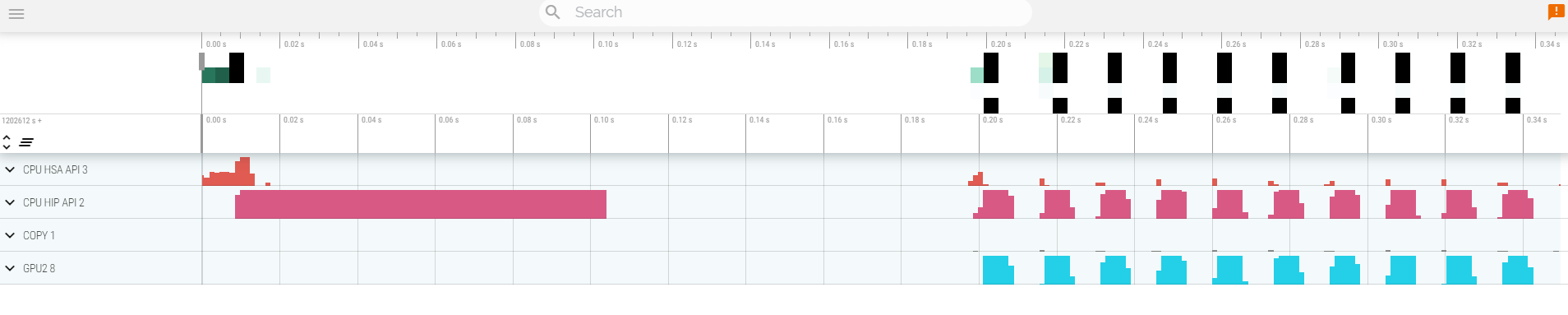
scp scp://USER@aac1.amd.com:<PORT>/~/HPCTrainingExamples/HIPIFY/mini-nbody/hip/results.json ./Open a browser and go to https://ui.perfetto.dev/. Click on Open trace file in the top left corner. Navigate to the results.json you just downloaded. Use WASD to navigate the GUI
Read about hardware counters available for the GPU on this system (look for gfx90a section)
less $ROCM_PATH/lib/rocprofiler/gfx_metrics.xmlCreate a rocprof_counters.txt file with the counters you would like to collect
vi rocprof_counters.txtContent for rocprof_counters.txt:
pmc : Wavefronts VALUInsts
pmc : SALUInsts SFetchInsts GDSInsts
pmc : MemUnitBusy ALUStalledByLDS
Execute with the counters we just added:
rocprof --timestamp on -i rocprof_counters.txt nbody-orig 65536You’ll notice that rocprof runs 3 passes, one for each set of counters we have in that file.
Contents of rocprof_counters.csv
cat rocprof_counters.csvexitSetup environment
module purge
module load omnitrace gcc/13List the various options and environment settings available for the omnitrace category:
omnitrace-avail --categories omnitraceTo add brief descriptions, use -bd option
omnitrace-avail -bd --categories omnitraceCreate a configuration file. This config file can then be modified to change options to see what you want in the Omnitrace profile. If you do not provide a path to the config file, it will generate one in the current directory ./omnitrace-config.cfg.
omnitrace-avail -G ~/omnitrace.cfgCreate an Omnitrace configuration file with description per option. Beware, this is quite verbose.
omnitrace-avail -G ~/omnitrace_all.cfg --allDeclare to use this configuration file. Only needed if you had provided a custom path and/or filename for the config file when you created it.
export OMNITRACE_CONFIG_FILE=~/omnitrace.cfgGo to the jacobi code in the examples repo:
cd ~/HPCTrainingExamples/HIP/jacobiCompile
makeExecute the binary to make sure it runs successfully: - Note: To get rid of Read -1, expected 4136, errno = 1 add --mca pml ucx --mca pml_ucx_tls ib,sm,tcp,self,cuda,rocm to the mpirun command line
mpirun -np 1 ./Jacobi_hip -g 1 1(WARNING) - this may in the current container Run the code with omnitrace to get runtime instrumentation. Time it to see overhead of dyninst loading all libraries in the beginning.
mpirun -np 1 omnitrace-instrument -- ./Jacobi_hip -g 1 1Check available functions to instrument using the --print-available functions option. Note, the --simulate option will not execute the binary.
mpirun -np 1 omnitrace-instrument -v 1 --simulate --print-available functions -- ./Jacobi_hip -g 1 1Create instrumented binary
omnitrace-instrument -o ./Jacobi_hip.inst -- ./Jacobi_hipExecuting the new instrumented binary, time it to see lower overhead:
mpirun -np 1 omnitrace-run -- ./Jacobi_hip.inst -g 1 1See the list of the instrumented GPU calls:
cat omnitrace-Jacobi_hip.inst-output/<TIMESTAMP>/roctracer-0.txtIf you get errors when you run an instrumented binary or when you run with dynamic instrumentation, add the following options --monochrome -v 2 --debug and try:
mpirun -np 1 omnitrace-run --monochrome -v 2 --debug -- ./Jacobi_hip.inst -g 1 1Copy the perfetto-trace-0.proto to your laptop, open the web page https://ui.perfetto.dev/
scp scp://USER@aac1.amd.com:<PORT>/~/HPCTrainingExamples/HIP/jacobi/omnitrace-Jacobi_hip.inst-output/TIMESTAMP/perfetto-trace-0.proto ./Click Open trace file and select the .proto file

See a list of all the counters
omnitrace-avail --allDeclare in your configuration file:
OMNITRACE_ROCM_EVENTS = GPUBusy,Wavefronts,MemUnitBusyCheck again:
grep OMNITRACE_ROCM_EVENTS $OMNITRACE_CONFIG_FILERun the instrumented binary, and visualize the Perfetto trace produced to see the hardware counters:
mpirun -np 1 omnitrace-run -- ./Jacobi_hip.inst -g 1 1Run the instrumented binary with multiple ranks. You’ll find multiple perfetto-trace-*.proto files, one for each rank.
mpirun -np 2 omnitrace-run -- ./Jacobi_hip.inst -g 2 1You can visualize them separately in Perfetto, or combine them using cat and visualize them in the same Perfetto window.
cat perfetto-trace-0.proto perfetto-trace-1.proto > allprocesses.protoSet the following in your configuration file:
OMNITRACE_USE_SAMPLING = true
OMNITRACE_SAMPLING_FREQ = 100
Execute the instrumented binary and visualize the perfetto trace.
mpirun -np 1 omnitrace-run -- ./Jacobi_hip.inst -g 1 1Scroll down to the very bottom to see the sampling output. Those traces will be annotated with a (S) as well.
Open the wall_clock-0.txt file:
cat omnitrace-Jacobi_hip.inst-output/<TIMESTAMP>/wall_clock-0.txtIn order to see the kernel durations aggregated in your configuration file, make sure to set in your config file or in the environment:
OMNITRACE_USE_TIMEMORY = true
OMNITRACE_FLAT_PROFILE = true
Execute the code and check the wall_clock-0.txt file again.
OMNITRACE_USE_TIMEMORY=true OMNITRACE_FLAT_PROFILE=true mpirun -np 1 omnitrace-run -- ./Jacobi_hip.inst -g 1 1Setup environment
module load rocm openmpiGet sample code
wget https://github.com/AMDResearch/omniperf/raw/main/sample/vcopy.cppCompile
hipcc -o vcopy vcopy.cppNOTE: THIS FAILS BECAUSE ROOFLINE CODE IS MISSING
Profile with omniperf
omniperf profile -n vcopy_all -- ./vcopy 1048576 256A new directory will be created named workloads/vcopy_all.
Analyze the collected profile using the built-in CLI
omniperf analyze -p workloads/vcopy_all/mi200/ &> vcopy_analyze.txtView vcopy_analyze.txt
less vcopy_analyze.txtWe can select specific IP Blocks to analyze
omniperf analyze -p workloads/vcopy_all/mi200/ -b 7.1.2If you’ve installed Omniperf on your laptop ( No ROCm Required ), you can download workloads/vcopy_all/mi200/ to your laptop and run omniperf with --gui option
omniperf analyze -p workloads/vcopy_all/mi200/ --guiOpen the following in your browser
http://172.21.7.117:8050/
cd HPCTrainingExamples/dgemm

mkdir build && cd build
cmake ..
make
Profile and analyze code
omniperf profile -n dgemm -- ./dgemm
omniperf analyze -p workloads/dgemm/mi200 >& omniperf.out
less omniperf.outSimple kernel implementing a version of yAx, to demonstrate effects of Launch Parameters on kernel execution time.
Note: This exercise was tested on a system with MI210s, on Omniperf version1.0.10 and ROCm 5.7.0, the section on the omniperf comparison feature currently requires building a release candidate that is newer than Omniperf 1.0.10.
The roofline model is a way to gauge kernel performance in terms of maximum achievable bandwidth and floating-point operations. It can be used to determine how efficiently a kernel makes use of the available hardware. It is a key tool in initially determining which kernels are performing well, and which kernels should be able to perform better. Below are roofline plots for the yAx kernel in problem.cpp:
| Roofline Type | Roofline Legend | Roofline Plot |
|---|---|---|
| FP32 |  |
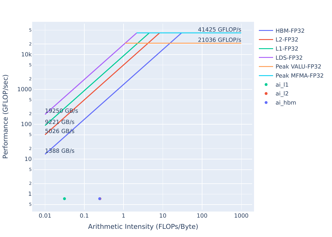 |
| FP16/INT8 | |
 |
These plots were generated by running:
omniperf profile -n problem_roof_only --roof-only --kernel-names -- ./problem.exeThe plots will appear as PDF files in the ./workloads/problem_roof_only/mi200 directory, if generated on MI200 hardware.
We see that the kernel’s performance is not near the achievable bandwidth possible on the hardware, which makes it a good candidate to consider optimizing.
From the roofline we were able to see that there is room for improvement in this kernel. One of the first things to check is whether or not we have reasonable launch parameters for this kernel.
To get started, build and run the problem code:
make
./problem.exe(simulated output)
yAx time: 2911 millisecondsThe runtime of the problem should be very slow, due to sub-optimal launch parameters. Let’s confirm this hypothesis by looking at the omniperf profile. Start by running:
omniperf profile -n problem --no-roof -- ./problem.exeThis command requires omniperf to run your code a few times to collect all the necessary hardware counters. - -n problem names the workload, meaning that the profile will appear in the ./workloads/problem/mi200/ directory, if you are profiling on an MI200 device. - --no-roof turns off the roofline, which will save some profiling time by avoiding the collection of achievable bandwidths and FLOPs on the device. - Everything after the -- is the command that will be profiled.
After the profiling data is collected, we can view the profile by using this command:
omniperf analyze -p workloads/problem/mi200 --dispatch 1 --metric 7.1.0 7.1.1 7.1.2This allows us to view nicely formatted profiling data directly in the command line. The command given here has a few arguments that are noteworthy: - -p workloads/problem/mi200 must point to the output directory of your profile run. For the above omniperf profile command, this will be workloads/problem/mi200. - --dispatch 1 filters kernel statistics by dispatch ID. In this case kernel 0 was a “warm-up” kernel, and kernel 1 is what the code reports timings for. - --metric displays only the requested metrics, in this case we want metrics specific to Launch Parameters: - 7.1.0 is the Grid Size - 7.1.1 is the Workgroup Size - 7.1.2 is the Total Wavefronts Launched
The output of the omniperf analyze command should look something like this:
--------
Analyze
--------


--------------------------------------------------------------------------------
0. Top Stat
----------------------------------------------------------------------------------------------------------------
|    | KernelName                               |   Count |      Sum(ns) |     Mean(ns) |   Median(ns) |    Pct |
----------------------------------------------------------------------------------------------------------------
|  0 | yax(double*, double*, double*, int, int, |    1.00 | 755935180.00 | 755935180.00 | 755935180.00 | 100.00 |
|    |  double*)                                |         |              |              |              |        |
----------------------------------------------------------------------------------------------------------------


--------------------------------------------------------------------------------
7. Wavefront
7.1 Wavefront Launch Stats
---------------------------------------------------------------------
| Index   | Metric           |    Avg |    Min |    Max | Unit       |
---------------------------------------------------------------------
| 7.1.0   | Grid Size        | 256.00 | 256.00 | 256.00 | Work items |
---------------------------------------------------------------------
| 7.1.1   | Workgroup Size   |  64.00 |  64.00 |  64.00 | Work items |
---------------------------------------------------------------------
| 7.1.2   | Total Wavefronts |   4.00 |   4.00 |   4.00 | Wavefronts |
---------------------------------------------------------------------
Looking through this data we see: - Workgroup Size (7.1.1) is 64 threads, which corresponds with the size of a wavefront. - Total Wavefronts (7.1.2) shows that we are launching only 4 Wavefronts.
We can definitely get better performance by adjusting the launch parameters of our kernel. Either try out some new values for the launch bounds, or run the provided solution to see its performance:
cd solution
make
./solution.exe(simulated output)
yAx time: 70 msWe get much better performance with the new launch parameters. Note that in general it can be difficult to find the most optimal launch parameters for a given kernel due to the many factors that impact performance, so determining launch parameters experimentally is usually necessary.
We should also confirm that our updated launch parameters are reported by omniperf, we need to run:
omniperf profile -n solution --no-roof -- ./solution.exeThis command is the same as before, except the workload name has changed to solution. Once the profile command has completed, run:
omniperf analyze -p workloads/solution/mi200 --dispatch 1 --metric 7.1.0 7.1.1 7.1.2Again, this command largely uses the same arguments as before, except for the workload name. The output should look something like this:
--------
Analyze
--------


--------------------------------------------------------------------------------
0. Top Stat
--------------------------------------------------------------------------------------------------------------
|    | KernelName                               |   Count |     Sum(ns) |    Mean(ns) |   Median(ns) |    Pct |
--------------------------------------------------------------------------------------------------------------
|  0 | yax(double*, double*, double*, int, int, |    1.00 | 70115217.00 | 70115217.00 |  70115217.00 | 100.00 |
|    |  double*)                                |         |             |             |              |        |
--------------------------------------------------------------------------------------------------------------


--------------------------------------------------------------------------------
7. Wavefront
7.1 Wavefront Launch Stats
------------------------------------------------------------------------------
| Index   | Metric           |       Avg |       Min |       Max | Unit       |
------------------------------------------------------------------------------
| 7.1.0   | Grid Size        | 131072.00 | 131072.00 | 131072.00 | Work items |
------------------------------------------------------------------------------
| 7.1.1   | Workgroup Size   |     64.00 |     64.00 |     64.00 | Work items |
------------------------------------------------------------------------------
| 7.1.2   | Total Wavefronts |   2048.00 |   2048.00 |   2048.00 | Wavefronts |
------------------------------------------------------------------------------
Looking through this data we see: - Workgroup Size (7.1.1) corresponds to the first argument of the block launch parameter - Total Wavefronts (7.1.2) corresponds to the first index of the grid launch parameter - Grid size (7.1.0) is Workgroup Size (7.1.1) times Total Wavefronts (7.1.2)
On releases newer than Omniperf 1.0.10, the comparison feature of omniperf can be used to quickly compare two profiles. To use this feature, use the command:
omniperf analyze -p workloads/problem/mi200 -p solution/workloads/solution/mi200 --dispatch 1 --metric 7.1.0 7.1.1 7.1.2This feature sets the first -p argument as the baseline, and the second as the comparison workload. In this case, problem is set as the baseline and is compared to solution. The output should look like:
--------
Analyze
--------


--------------------------------------------------------------------------------
0. Top Stat
-----------------------------------------------------------------------------------------------------------------------------------------------------------------------------------------------------------------
|    | KernelName                               |   Count | Count      |      Sum(ns) | Sum(ns)              |     Mean(ns) | Mean(ns)             |   Median(ns) | Median(ns)           |    Pct | Pct          |
-----------------------------------------------------------------------------------------------------------------------------------------------------------------------------------------------------------------
|  0 | yax(double*, double*, double*, int, int, |    1.00 | 1.0 (0.0%) | 754934306.50 | 69702016.5 (-90.77%) | 754934306.50 | 69702016.5 (-90.77%) | 754934306.50 | 69702016.5 (-90.77%) | 100.00 | 100.0 (0.0%) |
|    |  double*)                                |         |            |              |                      |              |                      |              |                      |        |              |
-----------------------------------------------------------------------------------------------------------------------------------------------------------------------------------------------------------------


--------------------------------------------------------------------------------
7. Wavefront
7.1 Wavefront Launch Stats
---------------------------------------------------------------------------------------------------------------------------------------
| Index   | Metric           |    Avg | Avg                 |    Min | Min                 |    Max | Max                 | Unit       |
---------------------------------------------------------------------------------------------------------------------------------------
| 7.1.0   | Grid Size        | 256.00 | 131072.0 (51100.0%) | 256.00 | 131072.0 (51100.0%) | 256.00 | 131072.0 (51100.0%) | Work items |
---------------------------------------------------------------------------------------------------------------------------------------
| 7.1.1   | Workgroup Size   |  64.00 | 64.0 (0.0%)         |  64.00 | 64.0 (0.0%)         |  64.00 | 64.0 (0.0%)         | Work items |
---------------------------------------------------------------------------------------------------------------------------------------
| 7.1.2   | Total Wavefronts |   4.00 | 2048.0 (51100.0%)   |   4.00 | 2048.0 (51100.0%)   |   4.00 | 2048.0 (51100.0%)   | Wavefronts |
---------------------------------------------------------------------------------------------------------------------------------------
Note that the comparison workload shows the percentage difference from the baseline. This feature can be used to quickly compare filtered stats to make sure code changes fix known issues.
For this exercise, it is appropriate to filter the omniperf analyze command with the --dispatch 1 argument. This --dispatch 1 argument filters the data shown to only include the kernel invocation with dispatch ID 1, or the second kernel run during profiling.
However, there is another way to filter kernels that may be more applicable in real use-cases. Typically real codes launch many kernels, and only a few of them take most of the overall kernel runtime. To see a ranking of the top kernels that take up most of the kernel runtime in your code, you can run:
omniperf analyze -p workloads/problem/mi200 --list-kernelsThis command will output something like:
--------
Analyze
--------


--------------------------------------------------------------------------------
Detected Kernels
----------------------------------------------------------
|    | KernelName                                        |
----------------------------------------------------------
|  0 | yax(double*, double*, double*, int, int, double*) |
----------------------------------------------------------
Using Omniperf versions greater than 1.0.10, --list-kernels will list all kernels launched by your code, in order of runtime (largest runtime first). The number displayed beside the kernel in the output can be used to filter omniperf analyze commands. Note that this will display aggregated stats for kernels of the same name, meaning that the invocations could differ in terms of launch parameters, and vary widely in terms of work completed. This filtering is accomplished with the -k argument:
omniperf analyze -p workloads/problem/mi200 -k 0 --metric 7.1.0 7.1.1 7.1.2Which should show something like:
--------
Analyze
--------


--------------------------------------------------------------------------------
0. Top Stat
-----------------------------------------------------------------------------------------------------------------------
|    | KernelName                               |   Count |       Sum(ns) |     Mean(ns) |   Median(ns) |    Pct | S   |
-----------------------------------------------------------------------------------------------------------------------
|  0 | yax(double*, double*, double*, int, int, |    2.00 | 1508098228.00 | 754049114.00 | 754049114.00 | 100.00 | *   |
|    |  double*)                                |         |               |              |              |        |     |
-----------------------------------------------------------------------------------------------------------------------


--------------------------------------------------------------------------------
7. Wavefront
7.1 Wavefront Launch Stats
----------------------------------------------------------------------
| Index   | Metric           |    Avg |    Min |    Max | Unit       |
----------------------------------------------------------------------
| 7.1.0   | Grid Size        | 256.00 | 256.00 | 256.00 | Work items |
----------------------------------------------------------------------
| 7.1.1   | Workgroup Size   |  64.00 |  64.00 |  64.00 | Work items |
----------------------------------------------------------------------
| 7.1.2   | Total Wavefronts |   4.00 |   4.00 |   4.00 | Wavefronts |
----------------------------------------------------------------------
Note that the ‘count’ field in Top Stat is 2 here, where filtering by dispatch ID displays a count of 1, indicating that filtering with -k returns aggregated stats for two kernel invocations in this case. Also note that the “Top Stats” table will still show all the top kernels but the rightmost column titled “S” will have an asterisk beside the kernel for which data is being displayed.
We’ve demonstrated better performance than problem.cpp in solution.cpp, but could we potentially do better? To answer that we again turn to the roofline model:
| Roofline Type | Roofline Legend | Roofline Plot |
|---|---|---|
| FP32 | |
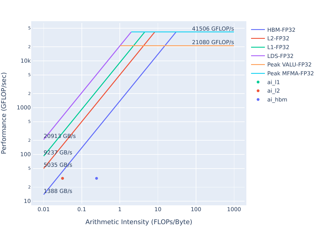 |
| FP16/INT8 | |
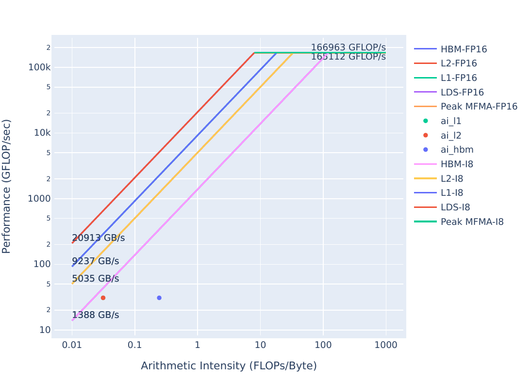 |
These plots were generated with:
omniperf profile -n solution_roof_only --roof-only --kernel-names -- ./solution.exeThe plots will appear as PDF files in the ./workloads/solution_roof_only/mi200 directory, if generated on MI200 hardware.
We see that the solution is solidly in the bandwidth-bound regime, but even still there seems to be room for improvement. Further performance improvements will be a topic for later exercises.
| Roofline Type | Problem Roofline | Solution Roofline |
|---|---|---|
| FP32 | |
|
| FP16/INT8 | |
|
We see that the solution has drastically increased performance over the problem code, as shown by the solution points moving up closer to the line plotted by the bandwidth limit.
Note: on statically generated roofline images, it is possible for the L1, L2, or HBM points to overlap and hide one another.
Launch parameters should be the first check in optimizing performance, due to the fact that they are usually easy to change, but can have a large performance impact if they aren’t tuned to your workload. It is difficult to predict the optimal launch parameters for any given kernel, so some experimentation may be required to achieve the best performance.
Simple kernel implementing a version of yAx, to demonstrate the downside of allocating a large amount of LDS, and the benefit of using a smaller amount of LDS due to occupancy limits.
Note: This exercise was tested on a system with MI210s, on omniperf version1.0.10 and ROCm 5.7.0
      <li><strong>FP(32/16):</strong> 32- or 16-bit Floating Point numeric types</li>
      <li><strong>FLOPs:</strong> Floating Point Operations Per second</li>
      <li><strong>HBM:</strong> High Bandwidth Memory is globally accessible from the GPU, and is a level of memory above the L2 cache</li>
</ul>In this exercise we’re using a problem code that is slightly different than where we left off in Exercise 1. Regardless, to get started we need to get a roofline by running:
omniperf profile -n problem_roof_only --roof-only --kernel-names -- ./problem.exeThe plots will appear as PDF files in the ./workloads/problem_roof_only/mi200 directory, if generated on MI200 hardware.
For convenience, the resulting plots on a representative system are below: | Roofline Type | Roofline Legend | Roofline Plot | |—————|—————————————————-|——————————————————| |FP32 ||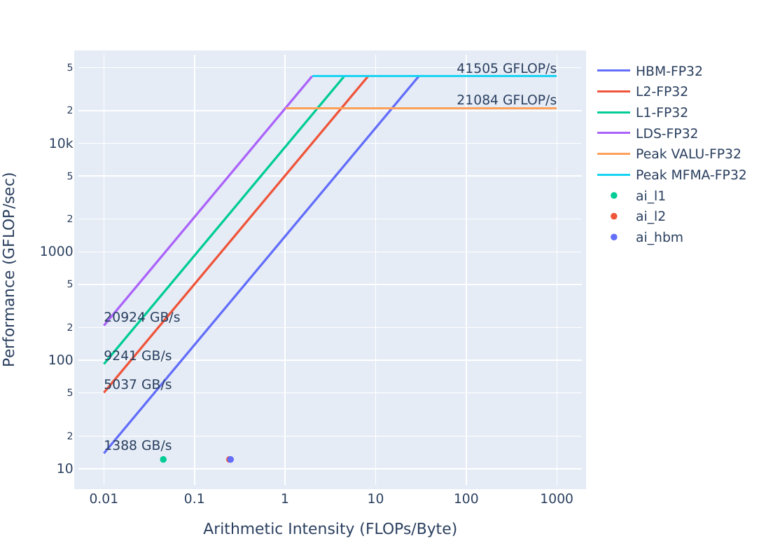 | |FP16/INT8 ||
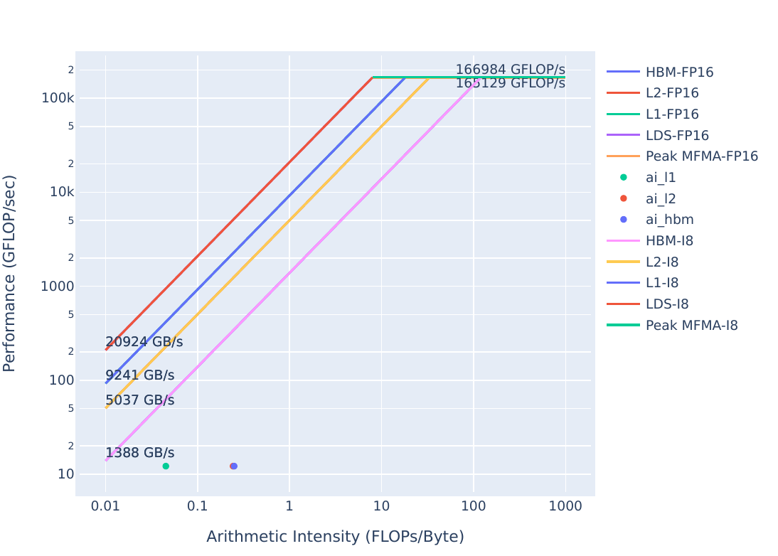 |
We see that there looks to be room for improvement here. We’ll use omniperf to see what the current limiters are.
First, we should get an idea of the code’s runtime:
make
./problem.exe(simulated output)
yAx time: 140 msThis problem.cpp uses LDS allocations to move the x vector closer to the compute resources, a common optimization. However, we see that it ends up slower than the previous solution that didn’t use LDS at all. In kernels that request a lot of LDS, it is common to see that the LDS usage limits the occupancy of the kernel. That is, more wavefronts cannot be resident on the device, because all of them need more LDS than is available. We need to confirm this hypothesis, let’s start by running:
omniperf profile -n problem --no-roof -- ./problem.exeThe usage of omniperf profile arguments can be found here, or by running omniperf profile --help.
This omniperf profile command will take a minute or two to run, as omniperf must run your code a few times to collect all the hardware counters.
Note: For large scientific codes, it can be useful to profile a small representative workload if possible, as profiling a full run may take prohibitively long.
Once the profiling run completes, let’s take a look at the occupancy stats related to LDS allocations:
omniperf analyze -p workloads/problem/mi200 --dispatch 1 --metric 2.1.26 6.2.7The metrics we’re looking at are: - 2.1.26 Wavefront occupancy – a measure of how many wavefronts, on average, are active on the device - 6.2.7 SPI: Insufficient CU LDS – indicates whether wavefronts are not able to be scheduled due to insufficient LDS
The SPI section (6.2) generally shows what resources limit occupancy, while Wavefront occupancy (2.1.26) shows how severely occupancy is limited in general. The SPI ‘insufficient’ fields are typically either zero or very large numbers (on the order of 1 million), with large numbers indicating some resource preventing wavefronts from scheduling. If more than one field is nonzero, the relative magnitude of the nonzero fields correspond to how severely the resources are limiting occupancy, but if only one field is nonzero it is difficult to say how severely that field is limiting occupancy.
The output of the omniperf analyze command should look similar to this:
--------
Analyze
--------


--------------------------------------------------------------------------------
0. Top Stat
-----------------------------------------------------------------------------------------------------------------
|    | KernelName                               |   Count |      Sum(ns) |     Mean(ns) |   Median(ns) |    Pct |
-----------------------------------------------------------------------------------------------------------------
|  0 | yax(double*, double*, double*, int, int, |    1.00 | 175427205.00 | 175427205.00 | 175427205.00 | 100.00 |
|    |  double*)                                |         |              |              |              |        |
-----------------------------------------------------------------------------------------------------------------


--------------------------------------------------------------------------------
2. System Speed-of-Light
2.1 Speed-of-Light
---------------------------------------------------------------------
| Index   | Metric         |   Value | Unit       |    Peak |   PoP |
---------------------------------------------------------------------
| 2.1.26  | Wave Occupancy |  102.70 | Wavefronts | 3328.00 |  3.09 |
---------------------------------------------------------------------


--------------------------------------------------------------------------------
6. Shader Processor Input (SPI)
6.2 SPI Resource Allocation
------------------------------------------------------------------------------------------
| Index   | Metric              |           Avg |           Min |           Max | Unit   |
------------------------------------------------------------------------------------------
| 6.2.7   | Insufficient CU LDS | 6015745446.00 | 6015745446.00 | 6015745446.00 | Cu     |
------------------------------------------------------------------------------------------
Looking through this data we see: - Wavefront occupancy (2.1.26) is 3%, which is very low - Insufficient CU LDS (6.2.7) contains a very large number, which indicates our occupancy is currently limited by LDS allocations.
There are two solution directories, which correspond to two ways that this occupancy limit can be addressed. First, we have solution-no-lds, which completely removes the LDS usage. Let’s build and run this solution:
cd solution-no-lds
make
./solution.exe(simulated output)
yAx time: 70 msWe see that the runtime is much better for this solution than the problem, let’s see if removing LDS did indeed increase occupancy:
omniperf profile -n solution --no-roof -- ./solution.exe(output omitted)
Once the profile command completes, run:
omniperf analyze -p workloads/solution/mi200 --dispatch 1 --metric 2.1.26 6.2.7The output should look something like:
--------
Analyze
--------


--------------------------------------------------------------------------------
0. Top Stat
--------------------------------------------------------------------------------------------------------------
|    | KernelName                               |   Count |     Sum(ns) |    Mean(ns) |   Median(ns) |    Pct |
--------------------------------------------------------------------------------------------------------------
|  0 | yax(double*, double*, double*, int, int, |    1.00 | 70512671.00 | 70512671.00 |  70512671.00 | 100.00 |
|    |  double*)                                |         |             |             |              |        |
--------------------------------------------------------------------------------------------------------------


--------------------------------------------------------------------------------
2. System Speed-of-Light
2.1 Speed-of-Light
---------------------------------------------------------------------
| Index   | Metric         |   Value | Unit       |    Peak |   PoP |
---------------------------------------------------------------------
| 2.1.26  | Wave Occupancy |  445.33 | Wavefronts | 3328.00 | 13.38 |
---------------------------------------------------------------------


--------------------------------------------------------------------------------
6. Shader Processor Input (SPI)
6.2 SPI Resource Allocation
------------------------------------------------------------------
| Index   | Metric              |   Avg |   Min |   Max | Unit   |
------------------------------------------------------------------
| 6.2.7   | Insufficient CU LDS |  0.00 |  0.00 |  0.00 | Cu     |
------------------------------------------------------------------
Looking through this data we see: - Wave occupancy (2.1.26) is 10% higher than in problem.cpp - Insufficient CU LDS (6.2.7) is now zero, indicating solution-no-lds is not occupancy limited by LDS allocations.
Can we get some runtime advantage from using smaller LDS allocations?
This is the solution implemented in the solution directory:
cd ../solution
make
./solution.exe(simulated output)
yAx time: 50 msThis solution, rather than removing the LDS allocation, simply reduces the amount of LDS requested to address the occupancy limit. This gives us the benefit of having some data pulled closer than it was in solution-no-lds which is validated through the speedup we see. But is this solution still occupancy limited by LDS?
omniperf profile -n solution --no-roof -- ./solution.exe(output omitted)
Once the profile command completes, run:
omniperf analyze -p workloads/solution/mi200 --dispatch 1 --metric 2.1.26 6.2.7The output should look something like:
--------
Analyze
--------


--------------------------------------------------------------------------------
0. Top Stat
--------------------------------------------------------------------------------------------------------------
|    | KernelName                               |   Count |     Sum(ns) |    Mean(ns) |   Median(ns) |    Pct |
--------------------------------------------------------------------------------------------------------------
|  0 | yax(double*, double*, double*, int, int, |    1.00 | 50366185.00 | 50366185.00 |  50366185.00 | 100.00 |
|    |  double*)                                |         |             |             |              |        |
--------------------------------------------------------------------------------------------------------------


--------------------------------------------------------------------------------
2. System Speed-of-Light
2.1 Speed-of-Light
---------------------------------------------------------------------
| Index   | Metric         |   Value | Unit       |    Peak |   PoP |
---------------------------------------------------------------------
| 2.1.26  | Wave Occupancy |  487.32 | Wavefronts | 3328.00 | 14.64 |
---------------------------------------------------------------------


--------------------------------------------------------------------------------
6. Shader Processor Input (SPI)
6.2 SPI Resource Allocation
------------------------------------------------------------------
| Index   | Metric              |   Avg |   Min |   Max | Unit   |
------------------------------------------------------------------
| 6.2.7   | Insufficient CU LDS |  0.00 |  0.00 |  0.00 | Cu     |
------------------------------------------------------------------
Looking at this data we see: - Wave Occupancy (2.1.26) is even higher than before - Insufficient CU LDS (6.2.7) shows we are not occupancy limited by LDS allocations.
Pulling some data from global device memory to LDS can be an effective optimization strategy, if occupancy limits are carefully avoided.
Let’s take a look at the roofline for solution, which can be generated with:
omniperf profile -n solution_roof_only --roof-only -- ./solution.exeThe plots will appear as PDF files in the ./workloads/problem_roof_only/mi200 directory, if generated on MI200 hardware.
The plots are shown here: | Roofline Type | Roofline Legend | Roofline Plot | |—————|—————————————————-|——————————————————| |FP32 ||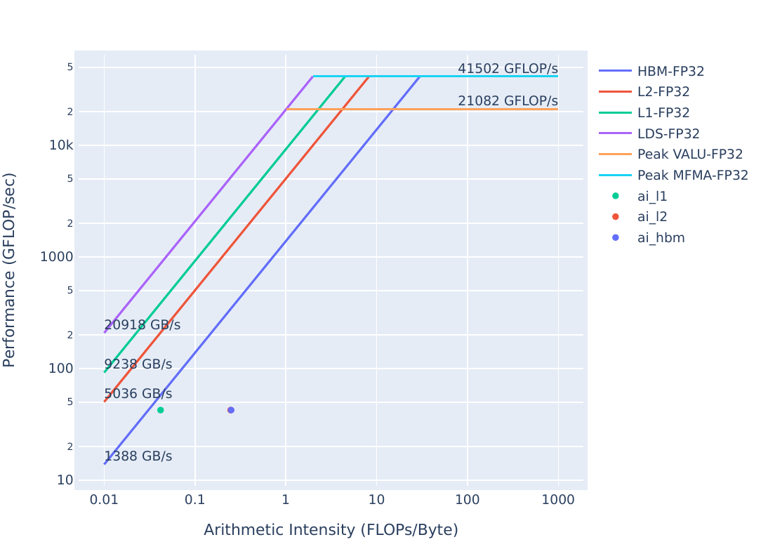 | |FP16/INT8 ||
 |
We see that there is still room to move the solution roofline up towards the bandwidth limit.
| Roofline Type | Problem Roofline | Solution Roofline |
|---|---|---|
| FP32 | |
|
| FP16/INT8 | |
|
Again, we see that the solution’s optimizations have resulted in the kernel moving up in the roofline, meaning the solution executes more efficiently than the problem.
Using LDS can be very helpful in reducing global memory reads where you have repeated use of the same data. However, large LDS allocations can also negatively impact performance by limiting the amount of wavefronts that can be resident in the device at any given time. Be wary of LDS usage, and check the SPI stats to ensure your LDS usage is not negatively impacting occupancy.
More complex yAx implementation to demonstrate a register limited kernel using an innocuous looking function call.
Note: This exercise was tested on a system with MI210s, on omniperf version1.0.10 and ROCm 5.7.0
      <li><strong>FP(32/16):</strong> 32- or 16-bit Floating Point numeric types</li>
      <li><strong>FLOPs:</strong> Floating Point Operations Per second</li>
      <li><strong>HBM:</strong> High Bandwidth Memory is globally accessible from the GPU, and is a level of memory above the L2 cache</li>
</ul>This kernel is slightly different from the one we used in previous exercises. Let’s see how well it measures up in the roofline:
| Roofline Type | Roofline Legend | Roofline Plot |
|---|---|---|
| FP32 | |
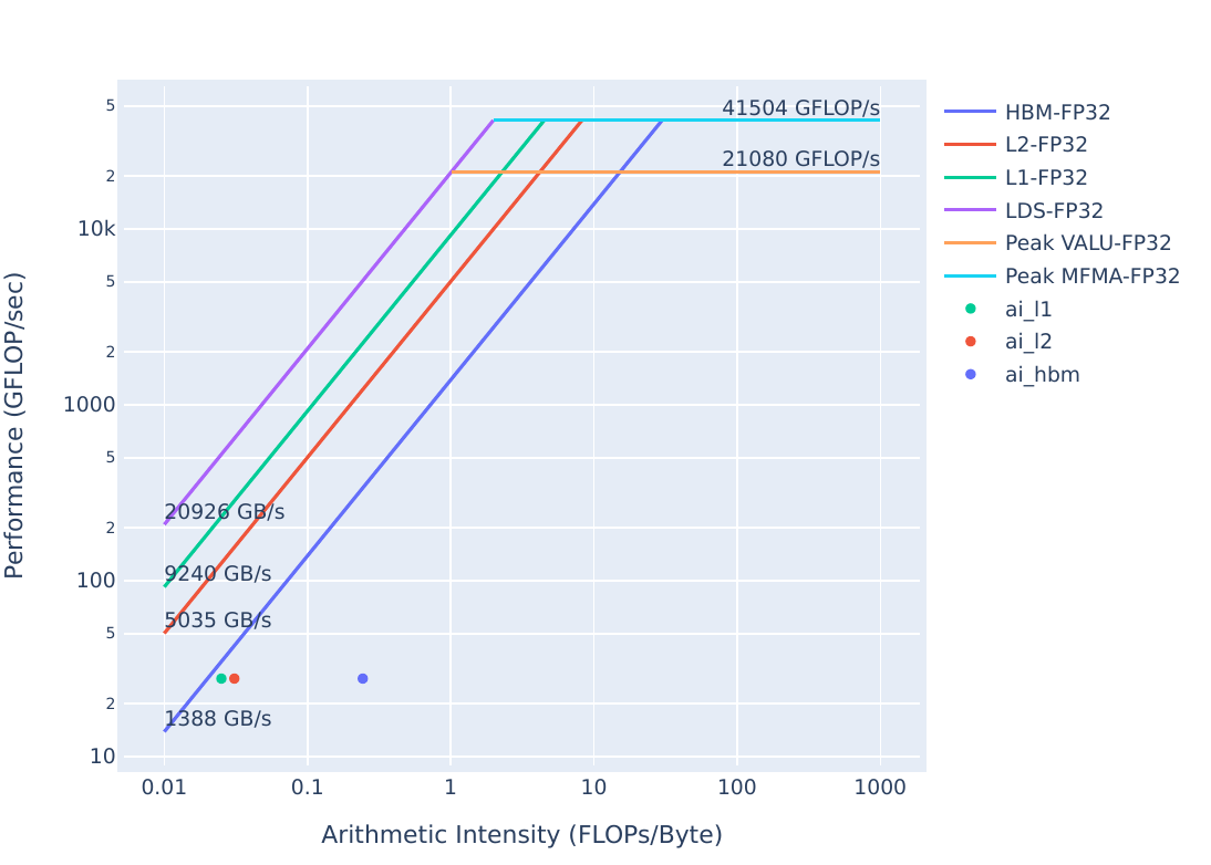 |
| FP16/INT8 | |
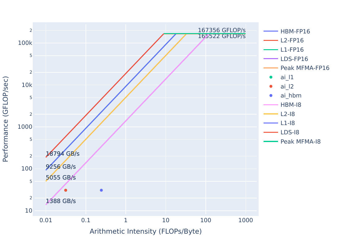 |
You can generate these plots by running:
omniperf profile -n problem_roof_only --roof-only --kernel-names -- ./problem.exeThe plots will appear as PDF files in the ./workloads/problem_roof_only/mi200 directory, if generated on MI200 hardware.
We see that the kernel is still a considerable amount below the maximum achievable bandwidth, so there should still be room for improvement.
Let’s get an idea of the runtime of this code:
make
./problem.exe(simulated output)
yAx time 79 msWe see that this kernel seems to be on par with some of our other exercises, but let’s see what omniperf shows us:
omniperf profile -n problem --no-roof -- ./problem.exe(lots of output from this command)
omniperf analyze -p workloads/problem/mi200 --dispatch 1 --metric 2.1.26 6.2.5 7.1.5 7.1.6 7.1.72.1.26 Shows Wavefront occupancy6.2.5 Shows Insufficient SIMD VGPRs – indicating if this kernel is occupancy limited by VGPR usage7.1.5-7 Shows the register usage: VGPRs, SGPRs, and AGPRs--------
Analyze
--------
--------------------------------------------------------------------------------
0. Top Stat
--------------------------------------------------------------------------------------------------------------
| | KernelName | Count | Sum(ns) | Mean(ns) | Median(ns) | Pct |
--------------------------------------------------------------------------------------------------------------
| 0 | yax(double*, double*, double*, int, int, | 1.00 | 76983902.00 | 76983902.00 | 76983902.00 | 100.00 |
| | double*) | | | | | |
--------------------------------------------------------------------------------------------------------------
--------------------------------------------------------------------------------
2. System Speed-of-Light
2.1 Speed-of-Light
--------------------------------------------------------------------
| Index | Metric | Value | Unit | Peak | PoP |
--------------------------------------------------------------------
| 2.1.26 | Wave Occupancy | 438.00 | Wavefronts | 3328.00 | 13.16 |
--------------------------------------------------------------------
--------------------------------------------------------------------------------
6. Shader Processor Input (SPI)
6.2 SPI Resource Allocation
----------------------------------------------------------------------------------------
| Index | Metric | Avg | Min | Max | Unit |
----------------------------------------------------------------------------------------
| 6.2.5 | Insufficient SIMD VGPRs | 13733460.00 | 13733460.00 | 13733460.00 | Simd |
----------------------------------------------------------------------------------------
--------------------------------------------------------------------------------
7. Wavefront
7.1 Wavefront Launch Stats
------------------------------------------------------------
| Index | Metric | Avg | Min | Max | Unit |
------------------------------------------------------------
| 7.1.5 | VGPRs | 92.00 | 92.00 | 92.00 | Registers |
------------------------------------------------------------
| 7.1.6 | AGPRs | 132.00 | 132.00 | 132.00 | Registers |
------------------------------------------------------------
| 7.1.7 | SGPRs | 48.00 | 48.00 | 48.00 | Registers |
------------------------------------------------------------Looking at this data, we see: - Insufficient SIMD VGPRs (6.2.5) shows a large number (on the order of 10 million), which indicates our kernel is occupancy limited by VGPR register usage. - VGPRs (7.1.5) shows we are using a lot of VGPRs and AGPRs (7.1.6) shows we are using a lot of AGPRs, which can indicate low-cost register spills in the absence of MFMA instructions.
This is due to a call to assert that checks if our result is zeroed out on device. We need to check this hypothesis, let’s look at the solution code:
cd solution
make
./solution.exe(simulated output)
yAx time: 70 msOur runtime gets better from removing the assert, but we should also check that omniperf reports that our limiters are gone:
omniperf profile -n solution --no-roof -- ./solution.exe(omitted output)
omniperf analyze -p workloads/solution/mi200 --dispatch 1 --metric 2.1.26 6.2.5 7.1.5 7.1.6 7.1.7The output of this command should look something like:
--------
Analyze
--------


--------------------------------------------------------------------------------
0. Top Stat
--------------------------------------------------------------------------------------------------------------
|    | KernelName                               |   Count |     Sum(ns) |    Mean(ns) |   Median(ns) |    Pct |
--------------------------------------------------------------------------------------------------------------
|  0 | yax(double*, double*, double*, int, int, |    1.00 | 69815871.00 | 69815871.00 |  69815871.00 | 100.00 |
|    |  double*)                                |         |             |             |              |        |
--------------------------------------------------------------------------------------------------------------


--------------------------------------------------------------------------------
2. System Speed-of-Light
2.1 Speed-of-Light
--------------------------------------------------------------------
| Index   | Metric         |   Value | Unit       |    Peak |   PoP |
--------------------------------------------------------------------
| 2.1.26  | Wave Occupancy |  444.10 | Wavefronts | 3328.00 | 13.34 |
--------------------------------------------------------------------


--------------------------------------------------------------------------------
6. Shader Processor Input (SPI)
6.2 SPI Resource Allocation
--------------------------------------------------------------------
| Index   | Metric                  |   Avg |   Min |   Max | Unit   |
--------------------------------------------------------------------
| 6.2.5   | Insufficient SIMD VGPRs |  0.00 |  0.00 |  0.00 | Simd   |
--------------------------------------------------------------------


--------------------------------------------------------------------------------
7. Wavefront
7.1 Wavefront Launch Stats
----------------------------------------------------------
| Index   | Metric   |   Avg |   Min |   Max | Unit      |
----------------------------------------------------------
| 7.1.5   | VGPRs    | 32.00 | 32.00 | 32.00 | Registers |
----------------------------------------------------------
| 7.1.6   | AGPRs    |  0.00 |  0.00 |  0.00 | Registers |
----------------------------------------------------------
| 7.1.7   | SGPRs    | 96.00 | 96.00 | 96.00 | Registers |
----------------------------------------------------------
Looking at this data, we see: - Insufficient SIMD VGPRs (6.2.5) shows we are no longer occupancy limited by VGPR usage. - VGPRs (7.1.5) and AGPRs (7.1.6) show considerably fewer vector registers, and no AGPRs being used. - SGPRs (7.1.7) shows a 2x increase over the previous implementation, which shows our memory access is more uniform here. - Wave Occupancy (2.1.26) shows our occupancy increased only slightly from the previous implementation, despite the large decrease in 6.2.5.
More generally, you can use this command to look at all SPI “insufficient resource” stats in the same screen, to determine if any resource is currently limiting occupancy:
omniperf analyze -p workloads/problem/mi200 --dispatch 1 --metric 6.2Which will show output similar to this (note, fields 6.2.4 to 6.2.9 show resources which currently limit occupancy):
--------
Analyze
--------


--------------------------------------------------------------------------------
0. Top Stat
---------------------------------------------------------------------------------------------------------------
|    | KernelName                               |   Count |     Sum(ns) |    Mean(ns) |   Median(ns) |    Pct |
---------------------------------------------------------------------------------------------------------------
|  0 | yax(double*, double*, double*, int, int, |    1.00 | 76983902.00 | 76983902.00 |  76983902.00 | 100.00 |
|    |  double*)                                |         |             |             |              |        |
---------------------------------------------------------------------------------------------------------------


--------------------------------------------------------------------------------
6. Shader Processor Input (SPI)
6.2 SPI Resource Allocation
------------------------------------------------------------------------------------------------
| Index   | Metric                      |         Avg |         Min |         Max | Unit        |
------------------------------------------------------------------------------------------------
| 6.2.0   | Wave request Failed (CS)    |   480983.00 |   480983.00 |   480983.00 | Cycles      |
------------------------------------------------------------------------------------------------
| 6.2.1   | CS Stall                    |   280093.00 |   280093.00 |   280093.00 | Cycles      |
------------------------------------------------------------------------------------------------
| 6.2.2   | CS Stall Rate               |        0.22 |        0.22 |        0.22 | Pct         |
------------------------------------------------------------------------------------------------
| 6.2.3   | Scratch Stall               |        0.00 |        0.00 |        0.00 | Cycles      |
------------------------------------------------------------------------------------------------
| 6.2.4   | Insufficient SIMD Waveslots |        0.00 |        0.00 |        0.00 | Simd        |
------------------------------------------------------------------------------------------------
| 6.2.5   | Insufficient SIMD VGPRs     | 13733460.00 | 13733460.00 | 13733460.00 | Simd        |
------------------------------------------------------------------------------------------------
| 6.2.6   | Insufficient SIMD SGPRs     |        0.00 |        0.00 |        0.00 | Simd        |
------------------------------------------------------------------------------------------------
| 6.2.7   | Insufficient CU LDS         |        0.00 |        0.00 |        0.00 | Cu          |
------------------------------------------------------------------------------------------------
| 6.2.8   | Insufficient CU Barries     |        0.00 |        0.00 |        0.00 | Cu          |
------------------------------------------------------------------------------------------------
| 6.2.9   | Insufficient Bulky Resource |        0.00 |        0.00 |        0.00 | Cu          |
------------------------------------------------------------------------------------------------
| 6.2.10  | Reach CU Threadgroups Limit |        0.00 |        0.00 |        0.00 | Cycles      |
------------------------------------------------------------------------------------------------
| 6.2.11  | Reach CU Wave Limit         |        0.00 |        0.00 |        0.00 | Cycles      |
------------------------------------------------------------------------------------------------
| 6.2.12  | VGPR Writes                 |        4.00 |        4.00 |        4.00 | Cycles/wave |
------------------------------------------------------------------------------------------------
| 6.2.13  | SGPR Writes                 |        3.00 |        3.00 |        3.00 | Cycles/wave |
------------------------------------------------------------------------------------------------Let’s see how the solution stacks up in the roofline:
| Roofline Type | Roofline Legend | Roofline Plot |
|---|---|---|
| FP32 | |
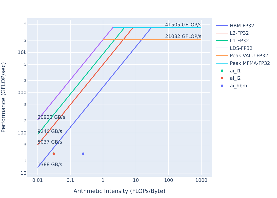 |
| FP16/INT8 | |
 |
You can generate these plots with:
omniperf profile -n problem_roof_only --roof-only --kernel-names -- ./problem.exeThe plots will appear as PDF files in the ./workloads/problem_roof_only/mi200 directory, if generated on MI200 hardware.
We see there is still room for improvement in the solution, as this kernel is not getting the maximum achievable bandwidth.
| Roofline Type | Problem Roofline | Solution Roofline |
|---|---|---|
| FP32 | |
|
| FP16/INT8 | |
|
The most notable change between these rooflines is that the L1/L2 arithmetic intensity spread is more pronounced in the problem, which shows that the call to assert was causing more data to be moved to the L1, while not adding floating-point operations.
Note: Arithmetic Intensity is computed as (total floating point operations)/(total data movement)
Function calls inside kernels can have surprisingly adverse performance side-effects. Calling assert, printf and even excessive use of math functions (e.g. pow, sin, cos) can limit performance in difficult-to-predict ways. If you see unexpected resource usage, try eliminating these sorts of function calls.
This exercise uses a simple implementation of a yAx kernel to show how difficult strided data access patterns can be to spot in code, and demonstrates how to use omniperf to begin to diagnose them.
Note: This exercise was tested on a system with MI210s, on omniperf version 1.0.10 and ROCm 5.7.0
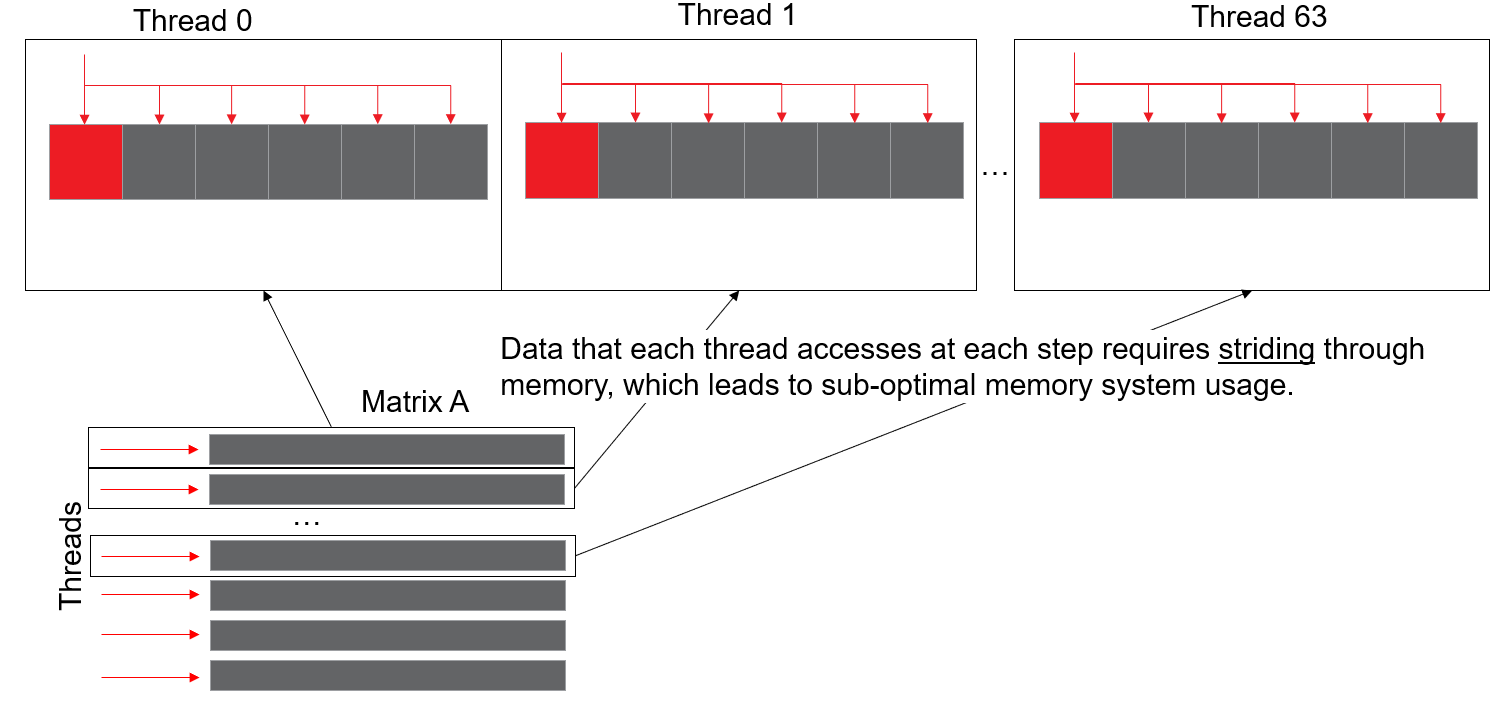 Here the memory addresses accessed by threads at each step of the computation have a lot of space between them, which is suboptimal for memory systems, especially on GPUs. To fix this, we have to re-structure the matrix A so that the columns of the matrix are contiguous, which will result in the rows striding, as seen below:
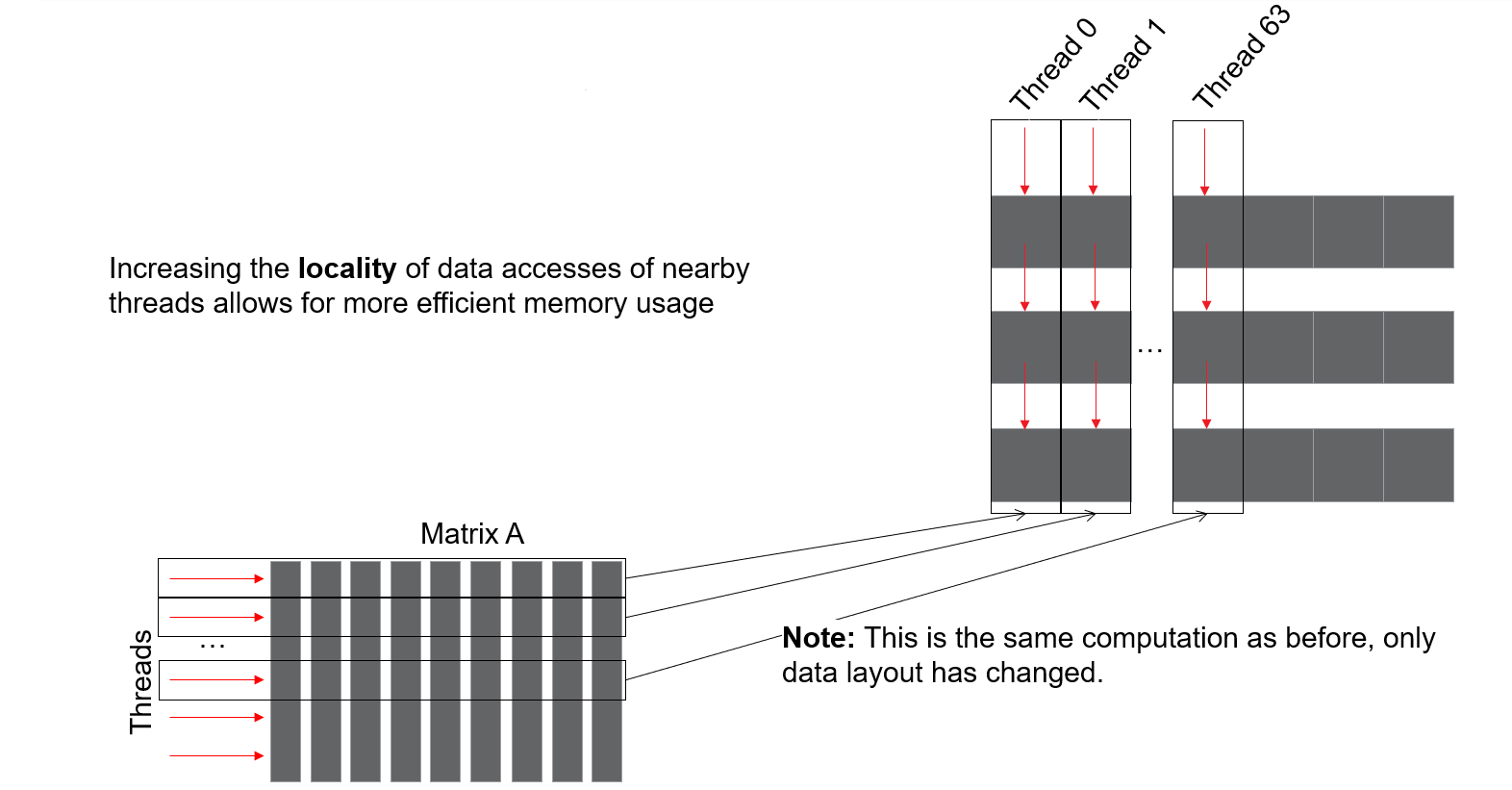 This new data layout has each block of threads accessing a contiguous chunk of device memory, and will use the memory system of the device much more efficiently. Importantly, the only thing that changed is the physical layout of the memory, so the result of this computation will be the same as the result of the previous data layout.
To start, we want to check the roofline of problem.exe, to make sure we are able to improve it. These plots can be generated with:
omniperf profile -n problem_roof_only --roof-only --kernel-names -- ./problem.exeThe plots will appear as PDF files in the ./workloads/problem_roof_only/mi200 directory, if generated on MI200 hardware.
They are also provided below for easy reference:
| Roofline Type | Roofline Legend | Roofline Plot |
|---|---|---|
| FP32 | |
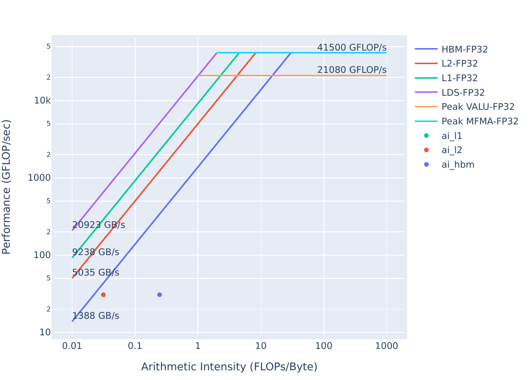 |
| FP16/INT8 | |
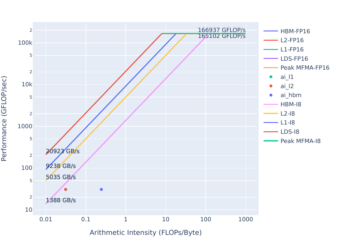 |
We have plenty of space to improve this kernel, the next step is profiling.
To start, let’s build and run the problem executable:
make
./problem.exe(simulated output)
yAx time: 70 msFrom our other experiments, this time seems reasonable. Let’s look closer at the memory system usage with omniperf:
omniperf profile -n problem --no-roof -- ./problem.exe(omitted output)
omniperf analyze -p workloads/problem/mi200 --dispatch 1 --metric 16.1 17.1Previous examples have used specific fields inside metrics, but we can also request a group of metrics with just two numbers (i.e. 16.1 vs. 16.1.1)
These requested metrics are: - 16.1 L1 memory speed-of-light stats - 17.1 L2 memory speed-of-light stats
The speed-of-light stats are a more broad overview of how the memory systems are used throughout execution of your kernel. As such, they’re great statistics for seeing if the memory system is generally being used efficiently or not. Output from the analyze command should look like this:
--------
Analyze
--------


--------------------------------------------------------------------------------
0. Top Stat
--------------------------------------------------------------------------------------------------------------
|    | KernelName                               |   Count |     Sum(ns) |    Mean(ns) |   Median(ns) |    Pct |
--------------------------------------------------------------------------------------------------------------
|  0 | yax(double*, double*, double*, int, int, |    1.00 | 69768072.00 | 69768072.00 |  69768072.00 | 100.00 |
|    |  double*)                                |         |             |             |              |        |
--------------------------------------------------------------------------------------------------------------


--------------------------------------------------------------------------------
16. Vector L1 Data Cache
16.1 Speed-of-Light
-------------------------------------------------------
| Index   | Metric            |   Value | Unit        |
-------------------------------------------------------
| 16.1.0  | Buffer Coalescing |   25.00 | Pct of peak |
-------------------------------------------------------
| 16.1.1  | Cache Util        |   87.79 | Pct of peak |
-------------------------------------------------------
| 16.1.2  | Cache BW          |    8.71 | Pct of peak |
-------------------------------------------------------
| 16.1.3  | Cache Hit         |    0.00 | Pct of peak |
-------------------------------------------------------


--------------------------------------------------------------------------------
17. L2 Cache
17.1 Speed-of-Light
-------------------------------------------
| Index   | Metric      |   Value | Unit   |
-------------------------------------------
| 17.1.0  | L2 Util     |   98.72 | Pct    |
-------------------------------------------
| 17.1.1  | Cache Hit   |   93.46 | Pct    |
-------------------------------------------
| 17.1.2  | L2-EA Rd BW |  125.87 | Gb/s   |
-------------------------------------------
| 17.1.3  | L2-EA Wr BW |    0.00 | Gb/s   |
-------------------------------------------
Looking at this data, we see: - L1 Cache Hit (16.1.3) is 0%, so the kernel’s memory requests are never found in the L1. - L2 Cache Hit (17.1.1) is 93.46%, so most requests are found in the L2, with about 7% needing to go out to HBM. - We are never finding data in the L1 and generating a lot of requests to the L2, so restructuring our data accesses should provide better performance
Since our implementation of yAx simply uses 1 for all values in y, A, and x, we do not have to change how we populate our data. Since A is implemented as a flat array, we don’t need to change our allocation either. >In real-world use-cases, these considerations add non-trivial development overhead, so data access patterns may be non-trivial to change.
To observe the performance effects of a different data access pattern, we simply need to change our indexing scheme. Let’s see how this performs by running solution:
cd solution
make
./solution.exe(simulated output)
yAx time: 12 msWe see the runtime here is significantly better than our previous kernel, but we need to check how the caches behave now:
omniperf profile -n solution --no-roof -- ./solution.exe(output omitted)
omniperf analyze -p workloads/solution/mi200 --dispatch 1 --metric 16.1 17.1The output from this analyze command should look like:
--------
Analyze
--------


--------------------------------------------------------------------------------
0. Top Stat
--------------------------------------------------------------------------------------------------------------
|    | KernelName                               |   Count |     Sum(ns) |    Mean(ns) |   Median(ns) |    Pct |
--------------------------------------------------------------------------------------------------------------
|  0 | yax(double*, double*, double*, int, int, |    1.00 | 12464570.00 | 12464570.00 |  12464570.00 | 100.00 |
|    |  double*)                                |         |             |             |              |        |
--------------------------------------------------------------------------------------------------------------


--------------------------------------------------------------------------------
16. Vector L1 Data Cache
16.1 Speed-of-Light
------------------------------------------------------
| Index   | Metric            |   Value | Unit        |
------------------------------------------------------
| 16.1.0  | Buffer Coalescing |   25.00 | Pct of peak |
------------------------------------------------------
| 16.1.1  | Cache Util        |   97.99 | Pct of peak |
------------------------------------------------------
| 16.1.2  | Cache BW          |   12.19 | Pct of peak |
------------------------------------------------------
| 16.1.3  | Cache Hit         |   49.98 | Pct of peak |
------------------------------------------------------


--------------------------------------------------------------------------------
17. L2 Cache
17.1 Speed-of-Light
-------------------------------------------
| Index   | Metric      |   Value | Unit   |
-------------------------------------------
| 17.1.0  | L2 Util     |   98.67 | Pct    |
-------------------------------------------
| 17.1.1  | Cache Hit   |    0.52 | Pct    |
-------------------------------------------
| 17.1.2  | L2-EA Rd BW |  689.26 | Gb/s   |
-------------------------------------------
| 17.1.3  | L2-EA Wr BW |    0.00 | Gb/s   |
-------------------------------------------
Looking at this data, we see: - L1 Cache Hit (16.1.3) is around 50%, so half the requests to the L1 need to go to the L2. - L2 Cache Hit (17.1.1) is 0.52%, so almost all the requests to the L2 have to go out to HBM. - L2-EA Rd BW (17.1.2) has increased significantly, due to the increase in L2 cache misses requiring HBM reads.
We should check where our new kernel stands on the roofline. These plots can be generated with:
omniperf profile -n solution_roof_only --roof-only --kernel-names -- ./solution.exeThe plots will appear as PDF files in the ./workloads/problem_roof_only/mi200 directory, if generated on MI200 hardware.
They are also provided below for easy reference:
| Roofline Type | Roofline Legend | Roofline Plot |
|---|---|---|
| FP32 | |
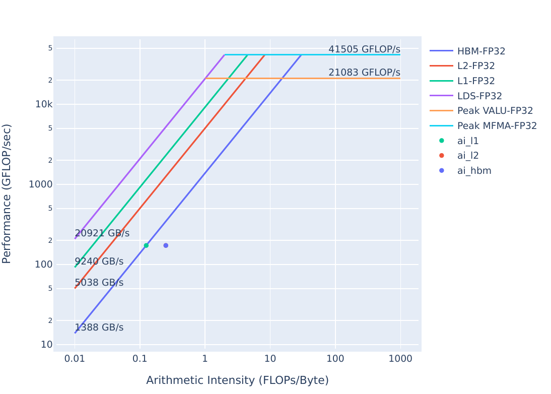 |
| FP16/INT8 | |
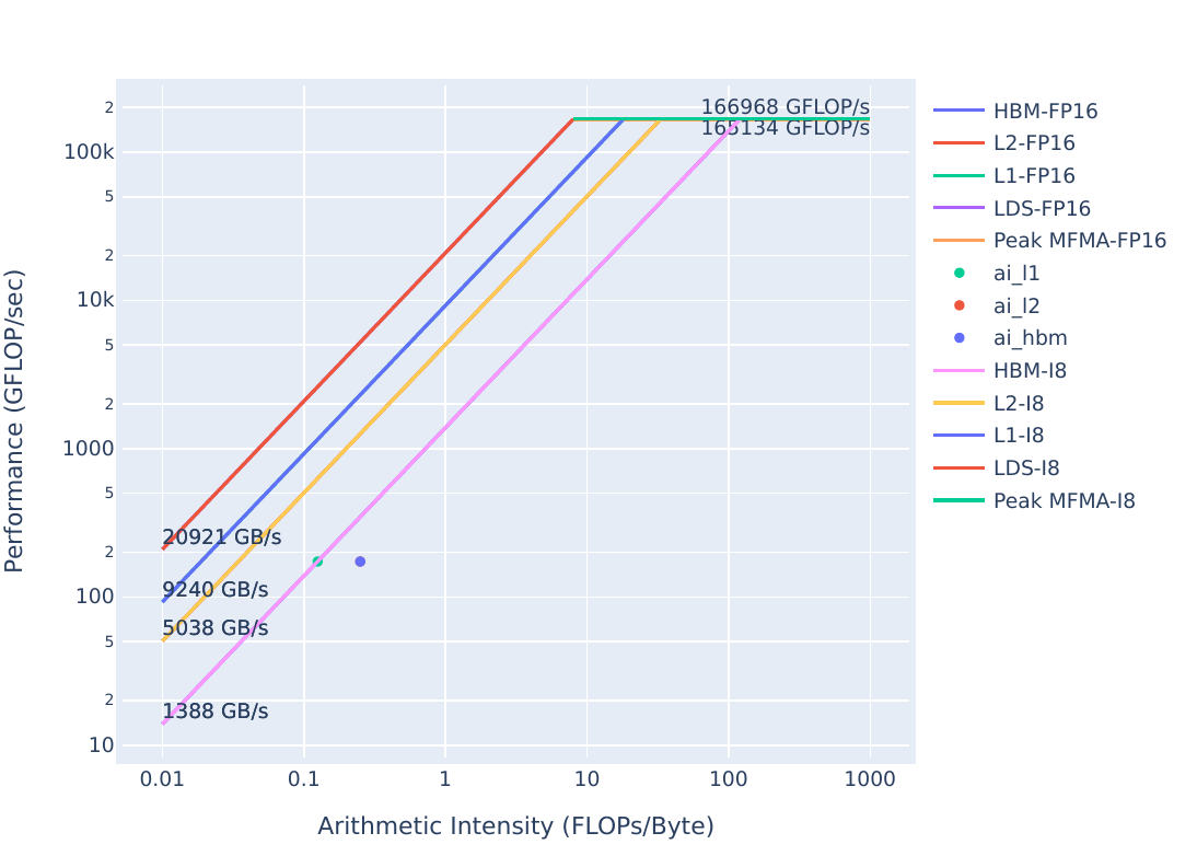 |
We appear to be very close to being bound by the HBM bandwidth from the fp32 roofline. To get more performance we need to look closer at our algorithm.
| Roofline Type | Problem Roofline | Solution Roofline |
|---|---|---|
| FP32 | |
|
| FP16/INT8 | |
|
We see that the HBM roofline point moves up, while the L1/L2 points move up and to the right from problem to solution. This means that our arithmetic intensity is increasing for the caches, so we are moving less data through the caches to do the same computation.
This exercise illustrates the at times insidious nature of strided data access patterns. They can be difficult to spot in code, but profiling more readily shows when adversarial access patterns occur, by showing poor cache hit rates, low cache bandwidth, and potentially low utilization. Data access patterns can be non-trivial to change, so these sorts of optimizations can involve significant development and validation overhead.
A simple yAx kernel, and more efficient, but more complex yAx kernel to demonstrate algorithmic improvements.
Note: This exercise was tested on a system with MI210s, on omniperf version 1.0.10 and ROCm 5.7.0
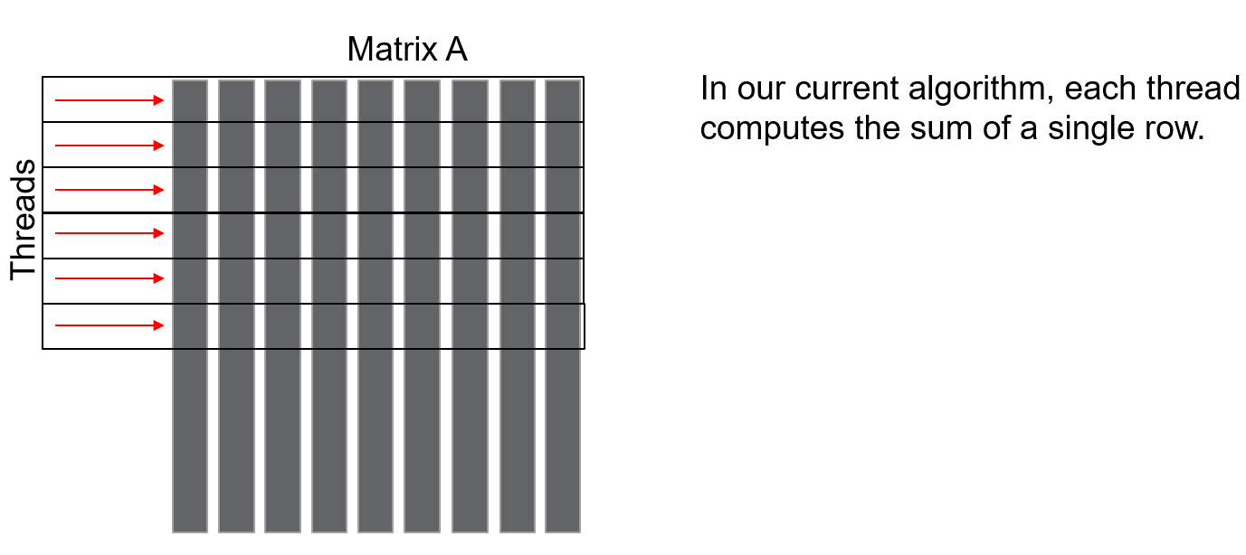 However, this is not efficient in the way the parallelism is expressed. Namely, we could add up all the partial sums for each row in parallel. This would make our approach to be: give a rows to wavefronts, and have the threads inside each wavefront sum up partial sums in parallel. Then, we reduce the partial sums atomically with shared memory, before completing the computation and reducing the final answer using global atomics. This approach expresses more of the parallelism that is available, and would look something like the figure below:
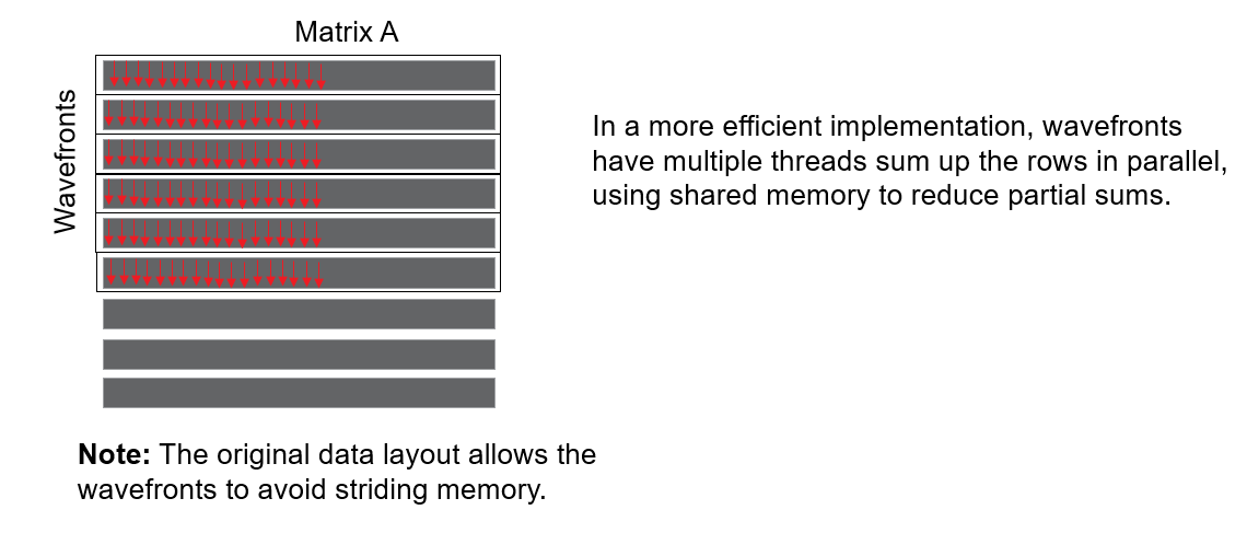 The expressed parallelism in each approach roughly corresponds to the number of red arrows in each figure.
We should start by doing a roofline to see where the problem executable stands. These plots can be generated with:
omniperf profile -n problem_roof_only --roof-only --kernel-names -- ./problem.exeThe plots will appear as PDF files in the ./workloads/problem_roof_only/mi200 directory, if generated on MI200 hardware.
They are also provided below for easy reference:
| Roofline Type | Roofline Legend | Roofline Plot |
|---|---|---|
| FP32 | |
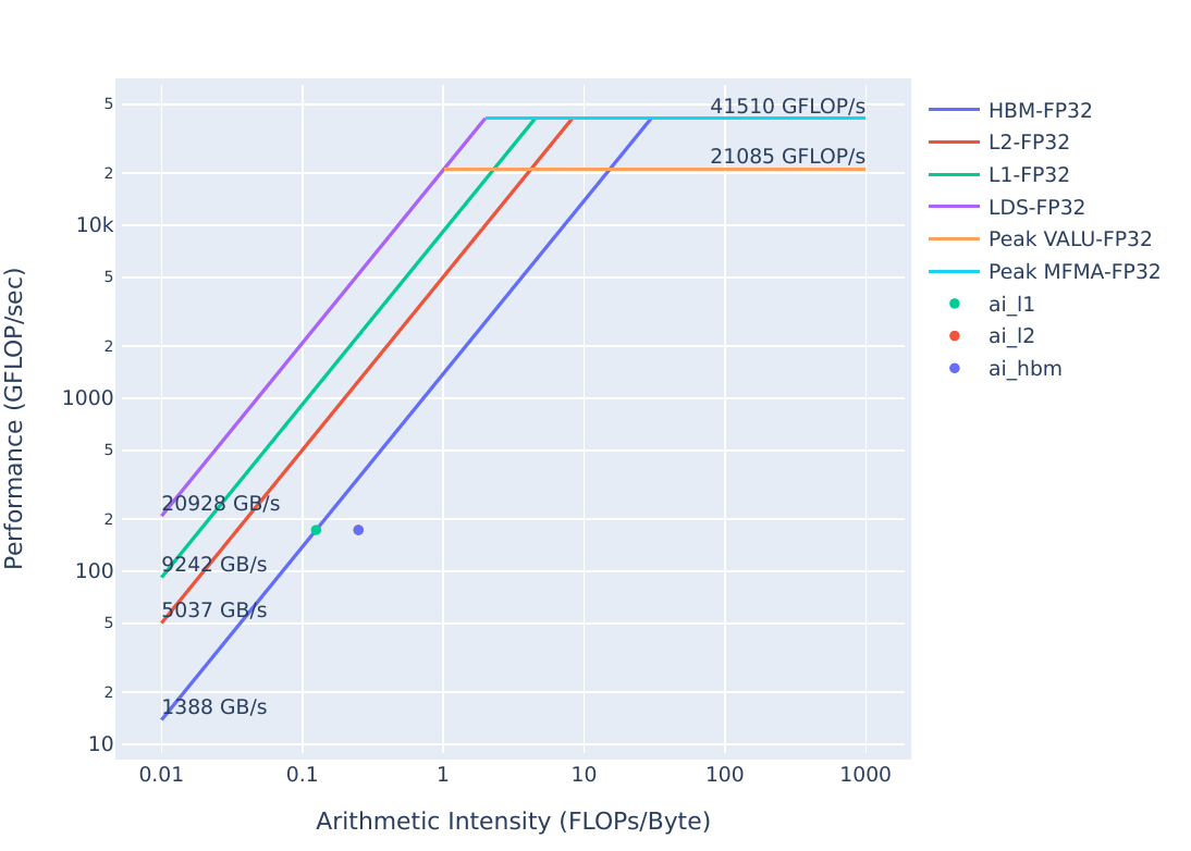 |
| FP16/INT8 | |
 |
The performance of this kernel looks pretty close to being HBM bandwidth bound. In the case of algorithmic optimizations, there may not be obvious evidence other than a suspicion that poor usage of hardware resources may be improved by changing the overall approach. In this case, we should be able to make better usage of both L1 and L2 resources by using wavefronts more efficiently to better parallelize our computation.
To start, let’s profile problem.exe:
make
./problem.exe(simulated output)
yAx time 12 msThis should be in line with our last solution. From the last exercise, we saw this output from omniperf analyze for this kernel:
--------
Analyze
--------


--------------------------------------------------------------------------------
0. Top Stat
---------------------------------------------------------------------------------------------------------------
|    | KernelName                               |   Count |     Sum(ns) |    Mean(ns) |   Median(ns) |    Pct |
---------------------------------------------------------------------------------------------------------------
|  0 | yax(double*, double*, double*, int, int, |    1.00 | 12427547.00 | 12427547.00 |  12427547.00 | 100.00 |
|    |  double*) [clone .kd]                    |         |             |             |              |        |
---------------------------------------------------------------------------------------------------------------


--------------------------------------------------------------------------------
16. Vector L1 Data Cache
16.1 Speed-of-Light
-----------------------------------------
| Index   | Metric            |   Value |
-----------------------------------------
| 16.1.0  | Buffer Coalescing |   25.00 |
-----------------------------------------
| 16.1.1  | Cache Util        |   98.19 |
-----------------------------------------
| 16.1.2  | Cache BW          |   12.22 |
-----------------------------------------
| 16.1.3  | Cache Hit         |   49.98 |
-----------------------------------------


--------------------------------------------------------------------------------
17. L2 Cache
17.1 Speed-of-Light
--------------------------------------------
| Index   | Metric      |   Value | Unit   |
--------------------------------------------
| 17.1.0  | L2 Util     |   98.45 | Pct    |
--------------------------------------------
| 17.1.1  | Cache Hit   |    0.52 | Pct    |
--------------------------------------------
| 17.1.2  | L2-EA Rd BW |  691.32 | Gb/s   |
--------------------------------------------
| 17.1.3  | L2-EA Wr BW |    0.00 | Gb/s   |
--------------------------------------------
Looking at this data again, we see: - L1 Cache Hit (16.1.3) is about 50%, which is fairly low for a “well performing” kernel. - L2 Cache Hit (17.1.1) is about 0%, which is very low to consider this kernel “well performing”.
Let’s run the profiling again, but dig more into detailed L1 and L2 stats to see if we can make better use of the L1 and L2:
omniperf profile -n problem --no-roof -- ./problem.exe(output omitted)
omniperf analyze -p workloads/problem/mi200 --dispatch 1 --metric 16.3 16.4 17.3 17.2The metrics we request are: - 16.3 Detailed L1 cache access stats - 16.4 Detailed L1-L2 transaction stats - 17.3 Detailed L2 access stats - 17.2 Detailed L2-Fabric transaction stats
The output from the analyze command should look something like:
--------
Analyze
--------


--------------------------------------------------------------------------------
0. Top Stat
--------------------------------------------------------------------------------------------------------------
|    | KernelName                               |   Count |     Sum(ns) |    Mean(ns) |   Median(ns) |    Pct |
--------------------------------------------------------------------------------------------------------------
|  0 | yax(double*, double*, double*, int, int, |    1.00 | 12392886.00 | 12392886.00 |  12392886.00 | 100.00 |
|    |  double*)                                |         |             |             |              |        |
--------------------------------------------------------------------------------------------------------------


--------------------------------------------------------------------------------
16. Vector L1 Data Cache
16.3 L1D Cache Accesses
----------------------------------------------------------------------------------------
| Index   | Metric              |        Avg |        Min |        Max | Unit           |
----------------------------------------------------------------------------------------
| 16.3.0  | Total Req           |  524368.00 |  524368.00 |  524368.00 | Req per wave   |
----------------------------------------------------------------------------------------
| 16.3.1  | Read Req            |  524304.00 |  524304.00 |  524304.00 | Req per wave   |
----------------------------------------------------------------------------------------
| 16.3.2  | Write Req           |       0.00 |       0.00 |       0.00 | Req per wave   |
----------------------------------------------------------------------------------------
| 16.3.3  | Atomic Req          |      64.00 |      64.00 |      64.00 | Req per wave   |
----------------------------------------------------------------------------------------
| 16.3.4  | Cache BW            |    1386.99 |    1386.99 |    1386.99 | Gb/s           |
----------------------------------------------------------------------------------------
| 16.3.5  | Cache Accesses      |  131140.00 |  131140.00 |  131140.00 | Req per wave   |
----------------------------------------------------------------------------------------
| 16.3.6  | Cache Hits          |   65538.00 |   65538.00 |   65538.00 | Req per wave   |
----------------------------------------------------------------------------------------
| 16.3.7  | Cache Hit Rate      |      49.98 |      49.98 |      49.98 | Pct            |
----------------------------------------------------------------------------------------
| 16.3.8  | Invalidate          |       0.00 |       0.00 |       0.00 | Req per wave   |
----------------------------------------------------------------------------------------
| 16.3.9  | L1-L2 BW            | 4198528.00 | 4198528.00 | 4198528.00 | Bytes per wave |
----------------------------------------------------------------------------------------
| 16.3.10 | L1-L2 Read          |   65538.00 |   65538.00 |   65538.00 | Req per wave   |
----------------------------------------------------------------------------------------
| 16.3.11 | L1-L2 Write         |       0.00 |       0.00 |       0.00 | Req per wave   |
----------------------------------------------------------------------------------------
| 16.3.12 | L1-L2 Atomic        |      64.00 |      64.00 |      64.00 | Req per wave   |
----------------------------------------------------------------------------------------
| 16.3.13 | L1 Access Latency   |     477.63 |     477.63 |     477.63 | Cycles         |
----------------------------------------------------------------------------------------
| 16.3.14 | L1-L2 Read Latency  |     399.51 |     399.51 |     399.51 | Cycles         |
----------------------------------------------------------------------------------------
| 16.3.15 | L1-L2 Write Latency |    5746.67 |    5746.67 |    5746.67 | Cycles         |
----------------------------------------------------------------------------------------
16.4 L1D - L2 Transactions
-----------------------------------------------------------------------------------------------
| Index   | Metric      | Xfer   | Coherency   |      Avg |      Min |      Max | Unit         |
-----------------------------------------------------------------------------------------------
| 16.4.0  | NC - Read   | Read   | NC          |     0.00 |     0.00 |     0.00 | Req per wave |
-----------------------------------------------------------------------------------------------
| 16.4.1  | UC - Read   | Read   | UC          |     0.00 |     0.00 |     0.00 | Req per wave |
-----------------------------------------------------------------------------------------------
| 16.4.2  | CC - Read   | Read   | CC          |     0.00 |     0.00 |     0.00 | Req per wave |
-----------------------------------------------------------------------------------------------
| 16.4.3  | RW - Read   | Read   | RW          | 65538.00 | 65538.00 | 65538.00 | Req per wave |
-----------------------------------------------------------------------------------------------
| 16.4.4  | RW - Write  | Write  | RW          |     0.00 |     0.00 |     0.00 | Req per wave |
-----------------------------------------------------------------------------------------------
| 16.4.5  | NC - Write  | Write  | NC          |     0.00 |     0.00 |     0.00 | Req per wave |
-----------------------------------------------------------------------------------------------
| 16.4.6  | UC - Write  | Write  | UC          |     0.00 |     0.00 |     0.00 | Req per wave |
-----------------------------------------------------------------------------------------------
| 16.4.7  | CC - Write  | Write  | CC          |     0.00 |     0.00 |     0.00 | Req per wave |
-----------------------------------------------------------------------------------------------
| 16.4.8  | NC - Atomic | Atomic | NC          |     0.00 |     0.00 |     0.00 | Req per wave |
-----------------------------------------------------------------------------------------------
| 16.4.9  | UC - Atomic | Atomic | UC          |     0.00 |     0.00 |     0.00 | Req per wave |
-----------------------------------------------------------------------------------------------
| 16.4.10 | CC - Atomic | Atomic | CC          |     0.00 |     0.00 |     0.00 | Req per wave |
-----------------------------------------------------------------------------------------------
| 16.4.11 | RW - Atomic | Atomic | RW          |    64.00 |    64.00 |    64.00 | Req per wave |
-----------------------------------------------------------------------------------------------


--------------------------------------------------------------------------------
17. L2 Cache
17.2 L2 - Fabric Transactions
-----------------------------------------------------------------------------------------
| Index   | Metric               | Avg        | Min        | Max        | Unit           |
-----------------------------------------------------------------------------------------
| 17.2.0  | Read BW              | 4195055.47 | 4195055.47 | 4195055.47 | Bytes per wave |
-----------------------------------------------------------------------------------------
| 17.2.1  | Write BW             | 0.14       | 0.14       | 0.14       | Bytes per wave |
-----------------------------------------------------------------------------------------
| 17.2.2  | Read (32B)           | 0.0        | 0.0        | 0.0        | Req per wave   |
-----------------------------------------------------------------------------------------
| 17.2.3  | Read (Uncached 32B)  | 0.55       | 0.55       | 0.55       | Req per wave   |
-----------------------------------------------------------------------------------------
| 17.2.4  | Read (64B)           | 65547.74   | 65547.74   | 65547.74   | Req per wave   |
-----------------------------------------------------------------------------------------
| 17.2.5  | HBM Read             | 65546.38   | 65546.38   | 65546.38   | Req per wave   |
-----------------------------------------------------------------------------------------
| 17.2.6  | Write (32B)          | 0.0        | 0.0        | 0.0        | Req per wave   |
-----------------------------------------------------------------------------------------
| 17.2.7  | Write (Uncached 32B) | 0.0        | 0.0        | 0.0        | Req per wave   |
-----------------------------------------------------------------------------------------
| 17.2.8  | Write (64B)          | 0.0        | 0.0        | 0.0        | Req per wave   |
-----------------------------------------------------------------------------------------
| 17.2.9  | HBM Write            | 0.01       | 0.01       | 0.01       | Req per wave   |
-----------------------------------------------------------------------------------------
| 17.2.10 | Read Latency         | 276.25     | 276.25     | 276.25     | Cycles         |
-----------------------------------------------------------------------------------------
| 17.2.11 | Write Latency        | 375.56     | 375.56     | 375.56     | Cycles         |
-----------------------------------------------------------------------------------------
| 17.2.12 | Atomic Latency       |            |            |            | Cycles         |
-----------------------------------------------------------------------------------------
| 17.2.13 | Read Stall           | 0.0        | 0.0        | 0.0        | Pct            |
-----------------------------------------------------------------------------------------
| 17.2.14 | Write Stall          | 0.0        | 0.0        | 0.0        | Pct            |
-----------------------------------------------------------------------------------------
17.3 L2 Cache Accesses
----------------------------------------------------------------------------------
| Index   | Metric             |      Avg |      Min |      Max | Unit            |
----------------------------------------------------------------------------------
| 17.3.0  | Req                | 32945.33 | 32945.33 | 32945.33 | Req per wave    |
----------------------------------------------------------------------------------
| 17.3.1  | Streaming Req      |     0.00 |     0.00 |     0.00 | Req per wave    |
----------------------------------------------------------------------------------
| 17.3.2  | Read Req           | 32881.34 | 32881.34 | 32881.34 | Req per wave    |
----------------------------------------------------------------------------------
| 17.3.3  | Write Req          |     0.00 |     0.00 |     0.00 | Req per wave    |
----------------------------------------------------------------------------------
| 17.3.4  | Atomic Req         |    64.00 |    64.00 |    64.00 | Req per wave    |
----------------------------------------------------------------------------------
| 17.3.5  | Probe Req          |     0.00 |     0.00 |     0.00 | Req per wave    |
----------------------------------------------------------------------------------
| 17.3.6  | Hits               |   171.59 |   171.59 |   171.59 | Hits per wave   |
----------------------------------------------------------------------------------
| 17.3.7  | Misses             | 32773.74 | 32773.74 | 32773.74 | Misses per wave |
----------------------------------------------------------------------------------
| 17.3.8  | Cache Hit          |     0.52 |     0.52 |     0.52 | Pct             |
----------------------------------------------------------------------------------
| 17.3.9  | Writeback          |     0.02 |     0.02 |     0.02 | per wave        |
----------------------------------------------------------------------------------
| 17.3.10 | NC Req             |     0.05 |     0.05 |     0.05 | Req per wave    |
----------------------------------------------------------------------------------
| 17.3.11 | UC Req             |     0.29 |     0.29 |     0.29 | Req per wave    |
----------------------------------------------------------------------------------
| 17.3.12 | CC Req             |     0.00 |     0.00 |     0.00 | Req per wave    |
----------------------------------------------------------------------------------
| 17.3.13 | RW Req             | 32945.00 | 32945.00 | 32945.00 | Req per wave    |
----------------------------------------------------------------------------------
| 17.3.14 | Writeback (Normal) |     0.00 |     0.00 |     0.00 | per wave        |
----------------------------------------------------------------------------------
| 17.3.15 | Writeback (TC Req) |     0.00 |     0.00 |     0.00 | per wave        |
----------------------------------------------------------------------------------
| 17.3.16 | Evict (Normal)     | 32742.27 | 32742.27 | 32742.27 | per wave        |
----------------------------------------------------------------------------------
| 17.3.17 | Evict (TC Req)     |     0.00 |     0.00 |     0.00 | per wave        |
----------------------------------------------------------------------------------
Profiling information of this level of detail is available, and it can be useful once it is determined that the high-level speed-of-light statistics indicate there may be a performance issue in the code that hits a specific hardware subsystem.
Looking at the L1 stats, we see: - L1 Total Req (16.3.0) and L1 Read Req (16.3.1) show we generate a lot of L1 requests - L1 Cache Hit Rate (16.3.7) shows half the requests have to go out to the L2
Looking at the L2 (17.3, 17.2) data, we see: - L2 Req (17.3.0) is 32945.33 - L2 Read Req (17.3.2) is 32881.84 - L2 Hits (17.3.6) is 171.59 - L2 Misses (17.3.7) is 32773.74 - We are issuing a lot of requests to the L2 (17.3.0,17.3.2), but we almost never find the data in the L2 (17.3.6, 17.3.7). - L2 Read Bandwidth (17.2.0) is consequently very high, the L2 always has to go out to HBM to find data.
This data indicates that we should be able to make better usage of our memory system, so let’s apply the algorithmic optimization present in solution.cpp:
cd solution
make
./solution.exe(simulated output)
yAx time: 0.4 msIt should be noted again that algorithmic optimizations are usually the most expensive optimizations to implement, as they usually entail re-conceptualizing the problem in a way that allows for a more efficient solution. However, as we see here, algorithmic optimization can result in impressive speedups. A better runtime is not proof that we are using our caches more efficiently, we have to profile the solution:
omniperf profile -n solution --no-roof -- ./solution.exe(output omitted)
omniperf analyze -p workloads/solution/mi200 --dispatch 1 --metric 16.3 16.4 17.3 17.2The output for the solution should look something like:
--------
Analyze
--------


--------------------------------------------------------------------------------
0. Top Stat
-----------------------------------------------------------------------------------------------------------
|    | KernelName                               |   Count |   Sum(ns) |   Mean(ns) |   Median(ns) |    Pct |
-----------------------------------------------------------------------------------------------------------
|  0 | yax(double*, double*, double*, int, int, |    1.00 | 415516.00 |  415516.00 |    415516.00 | 100.00 |
|    |  double*)                                |         |           |            |              |        |
-----------------------------------------------------------------------------------------------------------


--------------------------------------------------------------------------------
16. Vector L1 Data Cache
16.3 L1D Cache Accesses
----------------------------------------------------------------------------------
| Index   | Metric              |      Avg |      Min |      Max | Unit           |
----------------------------------------------------------------------------------
| 16.3.0  | Total Req           | 16448.00 | 16448.00 | 16448.00 | Req per wave   |
----------------------------------------------------------------------------------
| 16.3.1  | Read Req            | 16384.00 | 16384.00 | 16384.00 | Req per wave   |
----------------------------------------------------------------------------------
| 16.3.2  | Write Req           |     0.00 |     0.00 |     0.00 | Req per wave   |
----------------------------------------------------------------------------------
| 16.3.3  | Atomic Req          |    64.00 |    64.00 |    64.00 | Req per wave   |
----------------------------------------------------------------------------------
| 16.3.4  | Cache BW            |  1292.37 |  1292.37 |  1292.37 | Gb/s           |
----------------------------------------------------------------------------------
| 16.3.5  | Cache Accesses      |  4097.00 |  4097.00 |  4097.00 | Req per wave   |
----------------------------------------------------------------------------------
| 16.3.6  | Cache Hits          |  2864.00 |  2864.00 |  2864.00 | Req per wave   |
----------------------------------------------------------------------------------
| 16.3.7  | Cache Hit Rate      |    69.90 |    69.90 |    69.90 | Pct            |
----------------------------------------------------------------------------------
| 16.3.8  | Invalidate          |     0.00 |     0.00 |     0.00 | Req per wave   |
----------------------------------------------------------------------------------
| 16.3.9  | L1-L2 BW            | 78912.00 | 78912.00 | 78912.00 | Bytes per wave |
----------------------------------------------------------------------------------
| 16.3.10 | L1-L2 Read          |  1232.00 |  1232.00 |  1232.00 | Req per wave   |
----------------------------------------------------------------------------------
| 16.3.11 | L1-L2 Write         |     0.00 |     0.00 |     0.00 | Req per wave   |
----------------------------------------------------------------------------------
| 16.3.12 | L1-L2 Atomic        |     1.00 |     1.00 |     1.00 | Req per wave   |
----------------------------------------------------------------------------------
| 16.3.13 | L1 Access Latency   |   946.51 |   946.51 |   946.51 | Cycles         |
----------------------------------------------------------------------------------
| 16.3.14 | L1-L2 Read Latency  |   755.41 |   755.41 |   755.41 | Cycles         |
----------------------------------------------------------------------------------
| 16.3.15 | L1-L2 Write Latency |   875.86 |   875.86 |   875.86 | Cycles         |
----------------------------------------------------------------------------------
16.4 L1D - L2 Transactions
--------------------------------------------------------------------------------------------
| Index   | Metric      | Xfer   | Coherency   |     Avg |     Min |     Max | Unit         |
--------------------------------------------------------------------------------------------
| 16.4.0  | NC - Read   | Read   | NC          |    0.00 |    0.00 |    0.00 | Req per wave |
--------------------------------------------------------------------------------------------
| 16.4.1  | UC - Read   | Read   | UC          |    0.00 |    0.00 |    0.00 | Req per wave |
--------------------------------------------------------------------------------------------
| 16.4.2  | CC - Read   | Read   | CC          |    0.00 |    0.00 |    0.00 | Req per wave |
--------------------------------------------------------------------------------------------
| 16.4.3  | RW - Read   | Read   | RW          | 1232.00 | 1232.00 | 1232.00 | Req per wave |
--------------------------------------------------------------------------------------------
| 16.4.4  | RW - Write  | Write  | RW          |    0.00 |    0.00 |    0.00 | Req per wave |
--------------------------------------------------------------------------------------------
| 16.4.5  | NC - Write  | Write  | NC          |    0.00 |    0.00 |    0.00 | Req per wave |
--------------------------------------------------------------------------------------------
| 16.4.6  | UC - Write  | Write  | UC          |    0.00 |    0.00 |    0.00 | Req per wave |
--------------------------------------------------------------------------------------------
| 16.4.7  | CC - Write  | Write  | CC          |    0.00 |    0.00 |    0.00 | Req per wave |
--------------------------------------------------------------------------------------------
| 16.4.8  | NC - Atomic | Atomic | NC          |    0.00 |    0.00 |    0.00 | Req per wave |
--------------------------------------------------------------------------------------------
| 16.4.9  | UC - Atomic | Atomic | UC          |    0.00 |    0.00 |    0.00 | Req per wave |
--------------------------------------------------------------------------------------------
| 16.4.10 | CC - Atomic | Atomic | CC          |    0.00 |    0.00 |    0.00 | Req per wave |
--------------------------------------------------------------------------------------------
| 16.4.11 | RW - Atomic | Atomic | RW          |    1.00 |    1.00 |    1.00 | Req per wave |
--------------------------------------------------------------------------------------------


--------------------------------------------------------------------------------
17. L2 Cache
17.2 L2 - Fabric Transactions
-----------------------------------------------------------------------------------
| Index   | Metric               | Avg      | Min      | Max      | Unit           |
-----------------------------------------------------------------------------------
| 17.2.0  | Read BW              | 65688.72 | 65688.72 | 65688.72 | Bytes per wave |
-----------------------------------------------------------------------------------
| 17.2.1  | Write BW             | 0.02     | 0.02     | 0.02     | Bytes per wave |
-----------------------------------------------------------------------------------
| 17.2.2  | Read (32B)           | 0.0      | 0.0      | 0.0      | Req per wave   |
-----------------------------------------------------------------------------------
| 17.2.3  | Read (Uncached 32B)  | 0.27     | 0.27     | 0.27     | Req per wave   |
-----------------------------------------------------------------------------------
| 17.2.4  | Read (64B)           | 1026.39  | 1026.39  | 1026.39  | Req per wave   |
-----------------------------------------------------------------------------------
| 17.2.5  | HBM Read             | 1026.51  | 1026.51  | 1026.51  | Req per wave   |
-----------------------------------------------------------------------------------
| 17.2.6  | Write (32B)          | 0.0      | 0.0      | 0.0      | Req per wave   |
-----------------------------------------------------------------------------------
| 17.2.7  | Write (Uncached 32B) | 0.0      | 0.0      | 0.0      | Req per wave   |
-----------------------------------------------------------------------------------
| 17.2.8  | Write (64B)          | 0.0      | 0.0      | 0.0      | Req per wave   |
-----------------------------------------------------------------------------------
| 17.2.9  | HBM Write            | 0.0      | 0.0      | 0.0      | Req per wave   |
-----------------------------------------------------------------------------------
| 17.2.10 | Read Latency         | 700.24   | 700.24   | 700.24   | Cycles         |
-----------------------------------------------------------------------------------
| 17.2.11 | Write Latency        | 398.0    | 398.0    | 398.0    | Cycles         |
-----------------------------------------------------------------------------------
| 17.2.12 | Atomic Latency       |          |          |          | Cycles         |
-----------------------------------------------------------------------------------
| 17.2.13 | Read Stall           | 0.0      | 0.0      | 0.0      | Pct            |
-----------------------------------------------------------------------------------
| 17.2.14 | Write Stall          | 0.0      | 0.0      | 0.0      | Pct            |
-----------------------------------------------------------------------------------
17.3 L2 Cache Accesses
----------------------------------------------------------------------------
| Index   | Metric             |    Avg |    Min |    Max | Unit            |
----------------------------------------------------------------------------
| 17.3.0  | Req                | 617.41 | 617.41 | 617.41 | Req per wave    |
----------------------------------------------------------------------------
| 17.3.1  | Streaming Req      |   0.00 |   0.00 |   0.00 | Req per wave    |
----------------------------------------------------------------------------
| 17.3.2  | Read Req           | 616.41 | 616.41 | 616.41 | Req per wave    |
----------------------------------------------------------------------------
| 17.3.3  | Write Req          |   0.00 |   0.00 |   0.00 | Req per wave    |
----------------------------------------------------------------------------
| 17.3.4  | Atomic Req         |   1.00 |   1.00 |   1.00 | Req per wave    |
----------------------------------------------------------------------------
| 17.3.5  | Probe Req          |   0.00 |   0.00 |   0.00 | Req per wave    |
----------------------------------------------------------------------------
| 17.3.6  | Hits               | 104.03 | 104.03 | 104.03 | Hits per wave   |
----------------------------------------------------------------------------
| 17.3.7  | Misses             | 513.39 | 513.39 | 513.39 | Misses per wave |
----------------------------------------------------------------------------
| 17.3.8  | Cache Hit          |  16.85 |  16.85 |  16.85 | Pct             |
----------------------------------------------------------------------------
| 17.3.9  | Writeback          |   0.02 |   0.02 |   0.02 | per wave        |
----------------------------------------------------------------------------
| 17.3.10 | NC Req             |   0.03 |   0.03 |   0.03 | Req per wave    |
----------------------------------------------------------------------------
| 17.3.11 | UC Req             |   0.13 |   0.13 |   0.13 | Req per wave    |
----------------------------------------------------------------------------
| 17.3.12 | CC Req             |   0.00 |   0.00 |   0.00 | Req per wave    |
----------------------------------------------------------------------------
| 17.3.13 | RW Req             | 617.25 | 617.25 | 617.25 | Req per wave    |
----------------------------------------------------------------------------
| 17.3.14 | Writeback (Normal) |   0.00 |   0.00 |   0.00 | per wave        |
----------------------------------------------------------------------------
| 17.3.15 | Writeback (TC Req) |   0.00 |   0.00 |   0.00 | per wave        |
----------------------------------------------------------------------------
| 17.3.16 | Evict (Normal)     | 481.25 | 481.25 | 481.25 | per wave        |
----------------------------------------------------------------------------
| 17.3.17 | Evict (TC Req)     |   0.00 |   0.00 |   0.00 | per wave        |
----------------------------------------------------------------------------
Looking at the L1 data, we see: - L1 Cache Hit Rate (16.3.7) has increased about 20%. - L1 Total Req (16.3.0) has decreased by ~32x, 16448 compared to 524368 previously. - This results in fewer requests going out to the L2.
Looking at the L2 data, we see: - L2 Req (17.3.0) has decreased by ~53x, 617.4 compared to 32945.35 previously. - L2 Cache Hit (17.3.8) is orders of magnitude higher than before: 16.85% compared to 0.52% previously. - L2 Hits (17.3.6) is slightly lower than before: 104 compared to 171 - L2 Misses (17.3.7) has decreased by ~64x, 513 compared to 32773 - L2 Read bandwidth (17.2.0) has decreased due to the decrease in L2 misses. - We have orders of magnitude fewer requests going out to HBM than we did previously, which explains our observed speedup.
As a final step, we should check how this new implementation stacks up with the roofline. These plots can be generated with:
omniperf profile -n solution_roof_only --roof-only --kernel-names -- ./solution.exeThe plots will appear as PDF files in the ./workloads/solution_roof_only/mi200 directory, if generated on MI200 hardware.
They are also provided below for easy reference:
| Roofline Type | Roofline Legend | Roofline Plot |
|---|---|---|
| FP32 | |
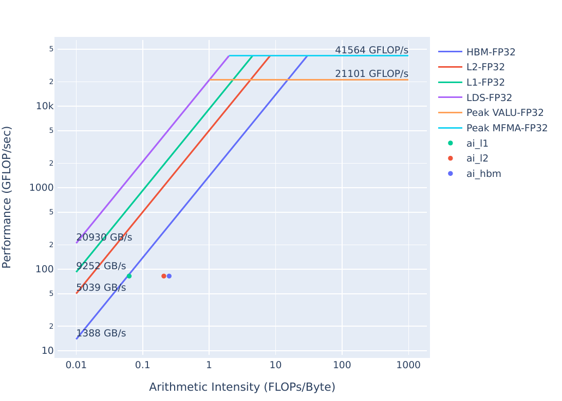 |
| FP16/INT8 | |
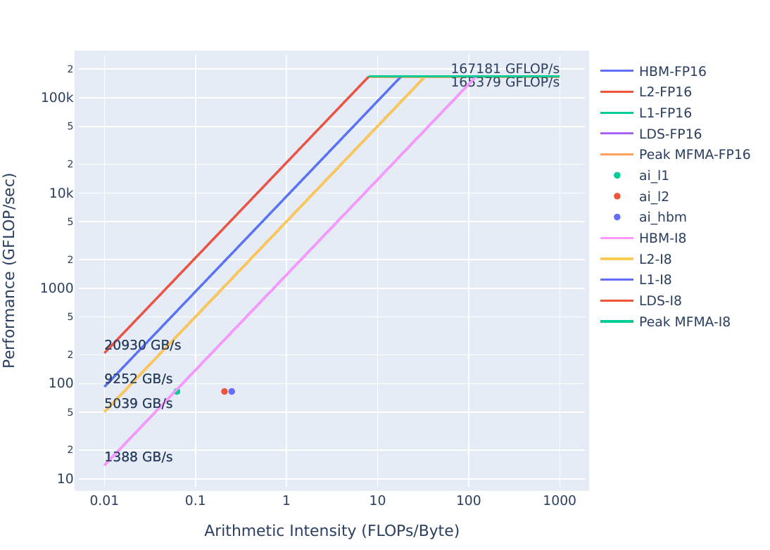 |
As the Omniperf stats indicate, we are moving most data through the L1, which shows in the roofline as a decrease in Arithmetic Intensity for that cache layer. We have a high hit rate in L1, with a fairly low hit rate in L2, and we end up having to go to HBM much less frequently than we did previously, thus our HBM bandwidth has decreased as a result of more efficient usage of our memory system.
The comparison of these two rooflines is confusing, due to the fact that these algorithms use the memory system very differently. It is important to keep in mind that our solution runs 29x faster than the problem.
| Roofline Type | Problem Roofline | Solution Roofline |
|---|---|---|
| FP32 | |
|
| FP16/INT8 | |
|
We see a significant speedup from problem to solution, but on the roofline it is difficult to determine which implementation is using the hardware more efficiently. The problem seems to be better, as the HBM point is very close to the achievable bandwidth, while the performance of the solution points seem to decrease. The roofline, though useful for estimating efficiencies of kernels, still only shows one perspective of performance.
This algorithmic optimization is able to work more efficiently out of the L1, generating far fewer L2 requests that require expensive memory operations. Algorithmic optimizations are all but guaranteed to have significant development overhead, but finding a more efficient algorithm can have large impacts to performance. If profiling reveals inefficient use of the memory hardware, it could be worth thinking about alternative algorithms.
The information presented in this document is for informational purposes only and may contain technical inaccuracies, omissions, and typographical errors. The information contained herein is subject to change and may be rendered inaccurate for many reasons, including but not limited to product and roadmap changes, component and motherboard version changes, new model and/or product releases, product differences between differing manufacturers, software changes, BIOS flashes, firmware upgrades, or the like. Any computer system has risks of security vulnerabilities that cannot be completely prevented or mitigated. AMD assumes no obligation to update or otherwise correct or revise this information. However, AMD reserves the right to revise this information and to make changes from time to time to the content hereof without obligation of AMD to notify any person of such revisions or changes.
THIS INFORMATION IS PROVIDED “AS IS.” AMD MAKES NO REPRESENTATIONS OR WARRANTIES WITH RESPECT TO THE CONTENTS HEREOF AND ASSUMES NO RESPONSIBILITY FOR ANY INACCURACIES, ERRORS, OR OMISSIONS THAT MAY APPEAR IN THIS INFORMATION. AMD SPECIFICALLY DISCLAIMS ANY IMPLIED WARRANTIES OF NON-INFRINGEMENT, MERCHANTABILITY, OR FITNESS FOR ANY PARTICULAR PURPOSE. IN NO EVENT WILL AMD BE LIABLE TO ANY PERSON FOR ANY RELIANCE, DIRECT, INDIRECT, SPECIAL, OR OTHER CONSEQUENTIAL DAMAGES ARISING FROM THE USE OF ANY INFORMATION CONTAINED HEREIN, EVEN IF AMD IS EXPRESSLY ADVISED OF THE POSSIBILITY OF SUCH DAMAGES.
Third-party content is licensed to you directly by the third party that owns the content and is not licensed to you by AMD. ALL LINKED THIRD-PARTY CONTENT IS PROVIDED “AS IS” WITHOUT A WARRANTY OF ANY KIND. USE OF SUCH THIRD-PARTY CONTENT IS DONE AT YOUR SOLE DISCRETION AND UNDER NO CIRCUMSTANCES WILL AMD BE LIABLE TO YOU FOR ANY THIRD-PARTY CONTENT. YOU ASSUME ALL RISK AND ARE SOLELY RESPONSIBLE FOR ANY DAMAGES THAT MAY ARISE FROM YOUR USE OF THIRD-PARTY CONTENT.
© 2023 Advanced Micro Devices, Inc. All rights reserved. AMD, the AMD Arrow logo, ROCm, Radeon, Radeon Instinct and combinations thereof are trademarks of Advanced Micro Devices, Inc. in the United States and/or other jurisdictions. Other names are for informational purposes only and may be trademarks of their